Out of order processor helps to improve ILP → find more independent
instructions to be executed
Improving ILP has been one of the main focuses in CPU designs.
Multi-threading: multiple HW threads with a PC and a register file
each
Amdahl's Law
P = parallel fraction (1-S)
N = number of processors (2, 4, 8, …)
S = serial fraction
Serial fraction is small (when S is close to 0), performance
improvement is proportional to N
Parallel Programming
Flynn’s Classical Taxonomy
SISD Single Instruction, Single Data
SIMD/SIMT Single Instruction, Multiple Data/Thread
MISD Multiple Instruction, Single Data
MIMD Multiple Instruction, Multiple Data
SPMD Programming
SPMD is typical GPU programming pattern and the hardware’s execution
model is SIMT.
Step 1: Discover Concurrency
Step 2: Structing the Algorithm
Step 3: Implementation
Step 4: Execution and Optimization
Parallel Programming
Patterns
1.Master/Worker Pattern
2.SPMD Pattern (Single Program, Multiple Data)
3.Loop Parallelism Pattern
4.Fork/Join Pattern
5.Pipeline Pattern
Programming with Shared
Memory
All processors can access the same memory
Proc 2 can observe updates made by Proc 1 by simply reading values
from shared memory.
Programming with
Distributed Memory
Distributed memory systems have each processor with its own memory
space
To access data in other memory space, processors send a message
Processor 2 requests messages from processor 1 and processor 3
OpenMP Programming
Parallelization
Specifying threads counts
Scheduling
Data Sharing
Synchronization
Mutex Operation
Mutex (mutual exclusion) ensures only one thread can access
critical section of code.
Lock: acquire a mutex to enter critical section
Unlock: release a mutex after finishing the critical section;
others are allowed to access the critical section
OpenMP Exp
1
2
3
4
5
6
7
8
9
10
11
12
intmain(){ constint size = 1000; // Size of the array int data[size]; // Initialize the array int sum = 0; #pragma omp parallel for reduction(+:sum) for (int i = 0; i < size; ++i) { sum += data[i]; } std::cout << "Sum of array elements: " << sum << std::endl; return0; }
Compiler directives
Works for C/C++/Fortran (used widely in HPC applications)
Compiler replaces directives with calls to runtime library
Library function handles thread create/join
#pragma omp directive [ clause [ clause ] … ]
Directives are the main OpenMP construct: pragrma omp parallel
for
Clauses provide additional information: reduction
(+:sum)
Reduction is commonly used.
Number of threads
by environment variable: OMP_NUM_THREADS
the omp_set_num_threads() function within the
code.
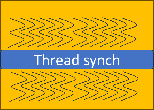
Thread Synchronization
Barrier: #pragma omp barrier
Synchronization point that all participating threads reach a
point
Green work won’t be started until all blue work is over.
#pragma omp parallel { #pragma omp for ordered for (int i = 0; i < 5; i++) { #pragma omp ordered { // This block of code will be executed in order printf(”Hello thread %d is doing iteration %d\n", omp_get_thread_num(), i); } } }
1 2 3 4 5 6 7 8 9
#pragma omp parallel { #pragma omp single { // This block of code will be executed by only one thread printf("This is a single thread task.\n"); } // Other parallel work... }
MPI Programming
MPI stands for message passing interface, a communication model for
parallel computing. Example: Two processes want to communicate with each
other.
Process 0 sends an integer value to process 1 using MPI_send();
Process 1 receives the value sent by process 0 using MPI_recv()
Broadcasting
Introducing MPI_Bcast(), a method to broadcast data from one process
to all other processes.
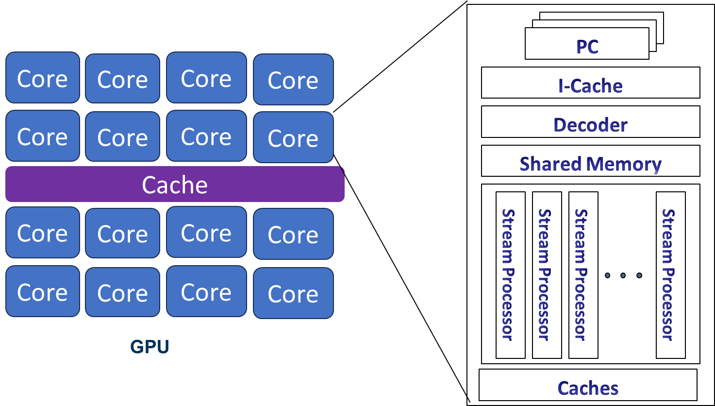
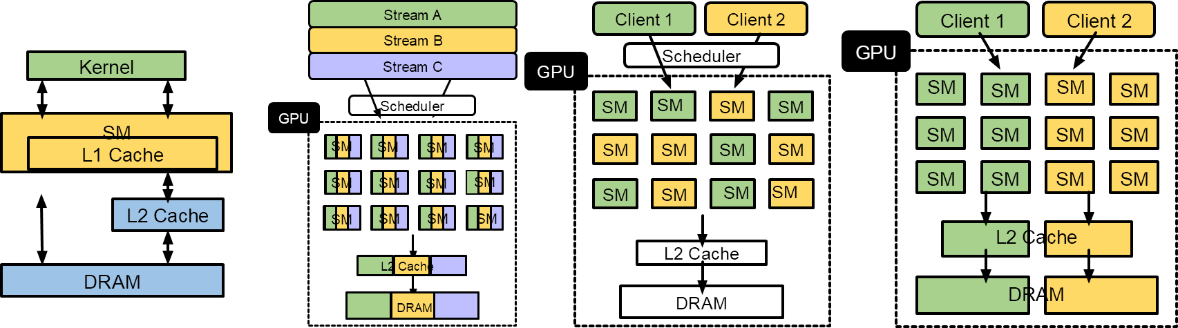
GPU Programming
GPU Architecture
Each core can execute multiple threads.
Stream processors are ALU units, SIMT lane or cores on GPUs
CPU Cores "Streaming multiprocessors(SM)" in NVIDIA term or SIMT
multiprocessors
Core ≠ stream processor
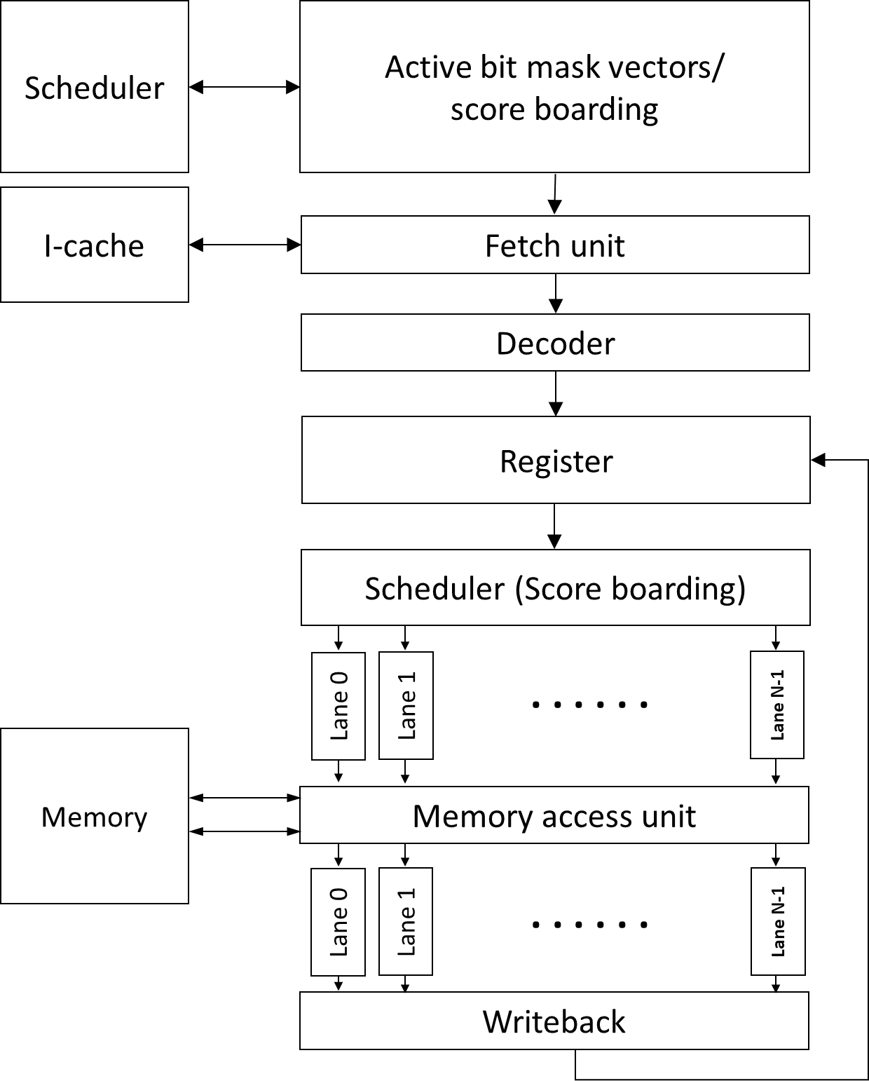
GPU Pipeline
Fetch
One instruction for each warp
Multiple PC registers exist to support multi-threaded
architecture
Round-robin scheduler
Greedy scheduler: switch warps on I-cache miss or branch
Decode
Register read
Scheduler (score boarding)
Execution (SIMT)
Writeback
Execution Unit:
Warp/Wave-front
Warp/wave-front is the basic unit of execution
A group of threads (e.g. 32 threads for the Tesla GPU
architecture)
Programmable GPU
Architecture Evolution
Cache hierarchies (L1, L2 etc.)
Extend FP 32 bits to FP 64 bits to support HPC
applications
Integration of atomic and fast integer operations to support more
diverse workloads
Supporting for PC per warp to PC per thread
Utilization of HBM memory (High bandwidth memory)
Addition of smaller floating points formats (FP16) to support ML
workloads. FP8 and other formats
Incorporation of tensor cores to support ML workloads
Integration of transformer cores to support transformer ML
workloads
CUDA Code Example: Vector
Add
1 2 3 4 5 6 7
__global__ voidvectorAdd(constfloat *A, constfloat *B, float *C, int numElements){ int i = blockDim.x * blockIdx.x + threadIdx.x; if (i < numElements) { C[i] = A[i] + B[i] + 0.0f; } }
1 2 3 4 5 6 7 8 9 10 11 12 13 14 15 16 17 18
intmain(void){
// Allocate the device input vector A float *d_A = NULL; err = cudaMalloc((void **)&d_A, size);
// Copy the host input vectors A and B in host memory to the device input // vectors in device memory printf("Copy input data from the host memory to the CUDA device\n"); err = cudaMemcpy(d_A, h_A, size, cudaMemcpyHostToDevice);
// Copy the device result vector in device memory to the host result vector // in host memory. printf("Copy output data from the CUDA device to the host memory\n"); err = cudaMemcpy(h_C, d_C, size, cudaMemcpyDeviceToHost); }
Host code is executed on CPUs
Kernel code is invoked with <<< …
>>>>
Kernel code is executed on GPUs
GPU kernel code is Single Program Multiple Data
All threads execute the same program.
There is no execution order among threads.
But we need to make each thread execute different data.
threadIdx.x
Even though each thread executes the same program
Now each thread has a unique identifier (each thread has built-in
variable that represents the x-axis coordinate).
Execution Hierarchy
A group of threads forms a block.
CUDA block: a group of threads that are executed
concurrently.
Data is divided by block.
For now, let’s just assume that each block is executed on each
GPU SM.
No ordering among CUDA block execution
1 2 3 4
vectorAdd (/* arguments should come here */) { int idx= blockIdx.x * blockDim.x + threadIdx.x; c[idx] = a[idx] + b[idx] }
Shared Memory
Scratchpad memory
Software controlled memory space
Use __shared__
On chip storage → faster access compared to global
memory
Accessible only within a CUDA block (later GPUs allow different
policy)
// Load data into shared memory __shared__ float sharedInput[sharedDim][sharedDim];
int sharedX = threadIdx.x + filterSize / 2; int sharedY = threadIdx.y + filterSize / 2;
//Load different values on boundaries if (x >= 0 && x < width && y >= 0 && y < height) { sharedInput[sharedY][sharedX] = input[y * width + x]; } else { sharedInput[sharedY][sharedX] = 0.0f; // Handle boundary conditions }
// Apply the filter to the pixel and its neighbors using shared memory for (int i = 0; i < filterSize; i++) { for (int j = 0; j < filterSize; j++) { result += sharedInput[threadIdx.y + i][threadIdx.x + j] * filter[i][j]; } }
OpenCL vs CUDA
OpenCL
CUDA
Execution Model
Work-groups/work-items
Block/Thread
Memory model
Global/constant/local/private
Global/constant/shared/local + Texture
Memory consistency
Weak consistency
Weak consistency
Synchronization
Synchronization using a work-group barrier (between work-items)
Using synch_threads Between threads
GPU Architecture
Multithreading
Benefits of Multithreading
Hide processor stall time:
Cache misses
Branch instructions
Long latency operations (ALU operations)
GPUs use multithreading to hide latency.
Out of order processors (OOO) use cache and ILP to hide
latency.
Longer memory latency requires a greater number of threads to hide
latency
Front-end Extension for
Multithreading
Multiple PC registers for Warps (one PC for each warp)
One static instruction for one warp (SPMD programming
model)
Individual registers for each thread
Minimizes context switch overhead
Significant resource
CPU Context Switching
CPU context switch: Store PC, architecture registers in
stack/memory
High overhead of CPU context switching
Hardware Support for
Multithreading
Front-end needs to have multiple PCs
One PC for each warp since all threads in a warp share the same
PC
Later GPUs have other advanced features
Large register file
Each thread needs “K” number of architecture registers
total register file size requirement = K times # number of
threads
“K” varies by applications
Remember occupancy calculation?
Each SM can execute Y number of threads, Z number of registers,
etc.
Y is related to # of PC registers
Z is related to K
Calculation Exp
Hardware example: SM can execute 256 threads, 64K registers, 32
KB shared memory; warp size is 32.
How many PCs are needed in one SM?
Answer: 256/32= 8 PCs
If a program has 10 instructions. How many times does one SM fetch
an instruction?
Answer: 10 x 8 = 80
CUDA Block/Threads/Warps
Multiple blocks can be running on one Multiprocessor.
Each block has multiple threads.
A group of threads are executed as a warp.
Registers are per thread.
Execution width x (2 source/1 write) registers accesses.
Port vs. Bank
Port: Hardware interface for data access
E.g., each thread requires 2 read and 1 write ports and execution
width is 4.
→ 8 read ports and 4 write ports
image-20251209005424492
Bank: a partition (group) of the register file
Multiple banks can be accessed simultaneously.
More ports mean more hardware wiring and resource usage
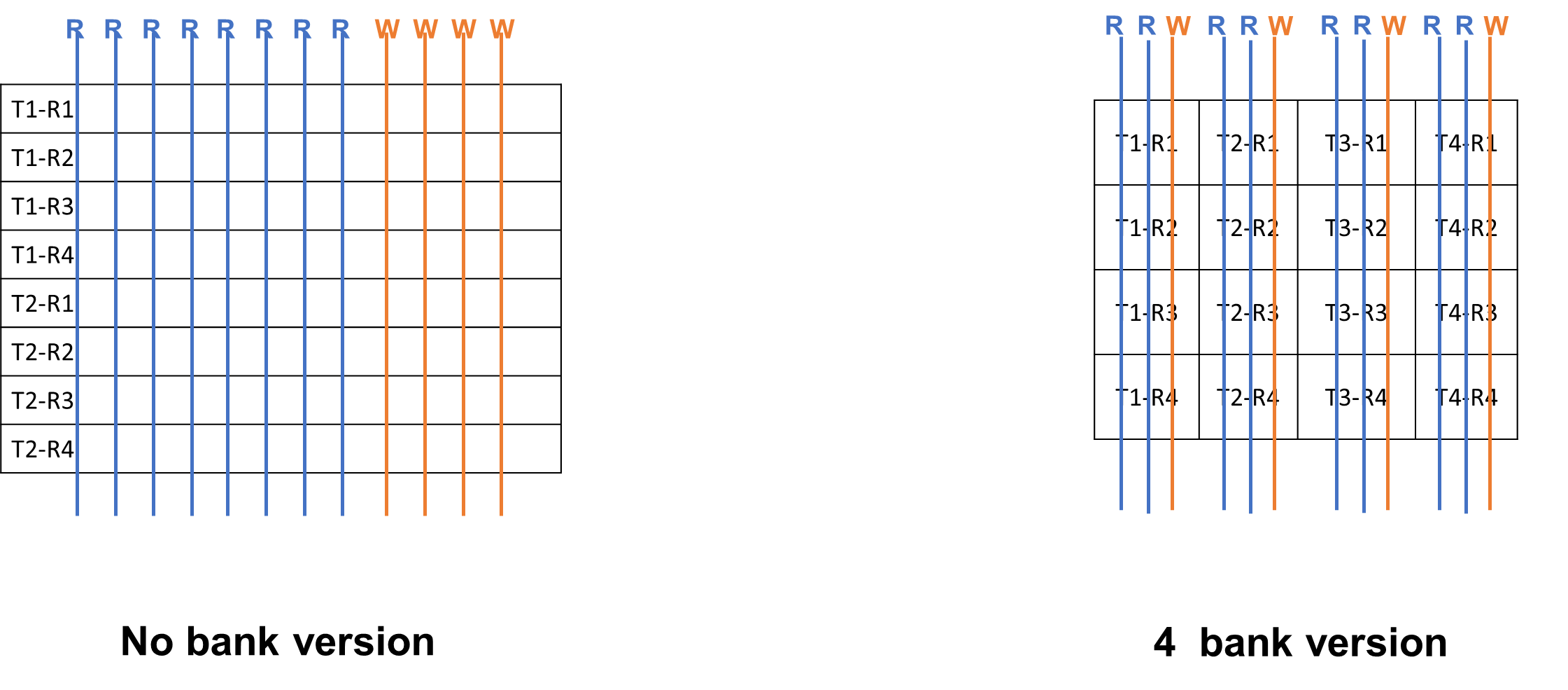
Variable Number of
Registers per Thread
CUDA programming will get benefits from different register counts
per thread
Instruction R3 = R1+R2
Case 1: 4 registers per 1 thread
Case 2: 2 registers per 1 thread
Case 1: reading registers would not cause a bank
conflict
Case 2: Read R1, R2 from multiple threads would cause a bank
conflict!
Remember: GPU executes a group of threads (warp), so multiple
threads are reading the same registers
Solution
Compiler-Driven solution for optimizing code layout
Register ID is known at static time.
Static vs. Dynamic
In this course, static often means
before running code. The property is not dependent on
input of the program. Dynamic means that the property
is dependent on input of the program.
E.g., static/dynamic number of instructions
1 2
LOOP: ADD R1 R1 #1 BREQ R1, 10, LOOP
Let’s say that loop iterates 10 times. Static number of
instructions is 2, dynamic number of instructions is 20.
Static time analysis = compile time analysis
Complexity beyond a 5-stage pipeline:
Register file access takes more than 1 cycle.
Source register values are buffered.
Scoreboarding
Widely used in CPU to enable out of order execution
Dynamic instruction scheduling
GPUs: check when all source operands within a warp are ready; the
warp is sent to execution units
Choose which one to send to the execution unit among multiple
warps
Even if the memory can provide high bandwidth memory, reducing
memory requests is critical.
GPU cache is very small.
image-20251209011252304
DRAM memory requests size is 64 ~ 128B
All memory requests from the first load can be combined into one
memory request mem[0]+28 → called coalesced.
Second load cannot be easily combined. → uncoalesced.
Coalesced Memory
Combining multiple memory requests into a single or more
efficient memory requests
Consecutive memory requests can be coalesced
Reduce the total number of memory requests
One of the key software optimization techniques
Program Pattern
Bank Conflict
Matrix Transpose
1
2
3
4
5
6
7
8
9
10
11
__global__ voidtransposeNaive(float *odata, constfloat *idata, int width, int height) { int x = blockIdx.x * blockDim.x + threadIdx.x; int y = blockIdx.y * blockDim.y + threadIdx.y;
if (x < width && y < height) { int input_idx = y * width + x; int output_idx = x * height + y; odata[output_idx] = idata[input_idx]; } }
Tile Version
1
2
3
4
5
6
7
8
9
__global__ voidtransposeNaive(float *odata, constfloat *idata) { int x = blockIdx.x * TILE_DIM + threadIdx.x; int y = blockIdx.y * TILE_DIM + threadIdx.y; int width = gridDim.x * TILE_DIM;
__global__ voidaccess(float* data, int width, int height){ int row = blockIdx.y * blockDim.y + threadIdx.y; int col = blockIdx.x * blockDim.x + threadIdx.x; int idx = col * height + row; data[idx] += 1.0f; }
What kind of memory access pattern does this kernel use within a
warp?
for (int offset = 16; offset > 0; offset /= 2) { val += __shfl_down_sync(FULL_MASK, val, offset); }
AtomicAdd & Cooperative
groups
1 2 3 4 5 6 7 8 9
__global__ voidreduce_atomic(float* data, int n, float* out){ int i = blockIdx.x * blockDim.x + threadIdx.x; float val = 0.0f; if (i < n) val = data[i];
FTZ: Flush-to-zero: round down (flush) to zero for very small
numbers (denormalized numbers)
RN: Round to nearest
Done by special Hardware in L2 cache (L1 caches are not
coherent!!)
Behavior is serialized.
Which of the following best describes the purpose of atomicAdd() in
CUDA?
A: "To perform a synchronized, conflict-free addition to a shared or
global memory location across many threads."
Programming Optimization
Cooperative Groups
Warp
A lock of execution
Width of warp →32.
What if we have work that require only fewer threads?
1 2
g.sync(); // synchronize group g cg::synchronize(g); // an equivalent way to synchronize g
1 2 3 4 5 6 7 8 9 10 11 12 13 14 15 16
usingnamespace cooperative_groups; __device__ intreduce_sum(thread_group g, int *temp, int val) { int lane = g.thread_rank(); //Rank is only unique within thread group
// Each iteration halves the number of active threads // Each thread adds its partial sum[i] to sum[lane+i] for (int i = g.size() / 2; i > 0; i /= 2) { temp[lane] = val; g.sync(); // wait for all threads to store if(lane<i) val += temp[lane + i]; g.sync(); // wait for all threads to load } return val; // note: only thread 0 will return full sum }
Let’s assume that an SM can execute 256 threads, and the width of a
warp is 8 threads. How many PCs are at least needed for one SM?
What is the primary purpose of mask bits in GPU architecture?
Mask bits indicate which threads (lanes) in a warp are active or
inactive during SIMT execution. They allow the GPU to selectively enable
or disable lanes when executing instructions, especially during branch
divergence.
cudaEventRecord (stop, 0); cudaEventSynchronize(stop); // make all work finished
Applications Suitable
for GPUs
Handle massive parallel data processing
Low Dominance in Host-Device Communication Costs
Coalesced Data Access (Global Memory Coalescing)
Profiling
Identify hotspots of applications
Measure key performance factors
Reported throughput
# of Divergent branches
# of Divergent memory (coalesced/uncoalesced)
Occupancy
Memory bandwidth utilizations
Use vendor-provided profiler to profile kernels
Optimization Techniques
Overall execution time = data transfer time + compute time +
memory access time
Data transfer time optimizations
Memory access pattern optimizations
Computation overhead reduction optimizations
Utilize libraries
Data Transfer Optimizations
Optimizations for data transfer between Host and Device
image-20251209204536403
Utilize fast transfer methods
E.g.) Pinned (page—locked) memory
Overlap Computation and Data Transfers
E.g.) cudaMemcpyAsync
Pipeline Transfer and Computation (Concurrent Copy and Execute)
E.g.) Use stream
Direct host memory access
Zero copy: access CPU data directly in the CPU and GPU integrated
memory
Unified virtual addressing (UVA)
Driver/runtime system hides the physically separated memory spaces
and provides an interface as if CPU and GPU can access any memory
Ideally no data copy cost but the implementation still requires data
copy and the overhead exists
Memory Access Pattern
Optimizations
Utilize caches
Global memory coalescing accesses
Aligned global memory accesses
Reducing the number of DRAM memory transactions is the
key
Check the average memory bandwidth
Reduce shared memory bank conflicts
Pinned/Page-Locked Host
Memory
Use CudaHostAlloc()
Operating system guarantees that the page resides in the system
in the Host side (Host has virtual memory) . Allows to access using a
physical memory access. --> allows GPU to use DMA to access CPU
memory (because it knows Physical memory addresses) → allows to achieve
the peak PCI-E bandwidth
Should we use all the time?
Size of (Pinned memory) < size of (physical memory)
Comparison code with cuda host
Reduce Computation Overhead
Instruction level optimizations
Replace with low-cost instructions
E.g.) Use shift operations instead of multiplication or
divisions
Use low precisions when possible (or use fewer number of
bits)
Use special hardware built-in special functions, e.g.,
rsqrtf()
Utilize Math libraries
Reduce branch statements
Use predicated execution if possible
Avoid atomic operations if possible
Use tensor operations and utilize tensor cores
New CUDA Features
Warp-level operations: warp shuffle/vote/ballot etc.
Communication between threads is expensive
Register files are unique to threads
Need to use shared memory which is expensive
Warp-level operations allow data movement withing a warp
Hardware support for warp level reduction
Cooperative groups
Instead of fixed warp size, smaller warp-level operations are
allowed
In the pinned memory style, which data structure needs to use
cudaHostAlloc? e.g.) copy from h_data (host data pointer) to d_data
(device data pointer)
A: The host-side buffer (h_data) must use
cudaHostAlloc() when using pinned-memory style. The device
pointer (d_data) is allocated with
cudaMalloc(), not cudaHostAlloc().
ft *h_x, *d_x[num_gpus], *d_y[num_gpus]; h_x = (ft *)malloc(ds * sizeof(ft));
for (int i = 0; i < num_gpus; i++) { cudaSetDevice(i); cudaMalloc(&d_x[i], ds * sizeof(ft)); // Malloc for each GPU cudaMalloc(&d_y[i], ds * sizeof(ft)); // Malloc for each GPU } cudaCheckErrors("allocation error");
for (int i = 0; i < num_gpus; i++) { for (size_t j = 0; j < ds; j++) { h_x[j] = rand() / (ft)RAND_MAX; } cudaSetDevice(i); // Indicate which device to use from the host side cudaMemcpy(d_x[i], h_x, ds * sizeof(ft), cudaMemcpyHostToDevice); } cudaCheckErrors("copy error");
unsignedlonglong et1 = dtime_usec(0);
for (int i = 0; i < num_gpus; i++) { cudaSetDevice(i); gaussian_pdf<<<(ds+255)/256, 256>>>(d_x[i], d_y[i], 0.0, 1.0, ds); // Kernel invocation for each GPU } cudaDeviceSynchronize(); // Wait until all devices finish cudaCheckErrors("execution error"); }
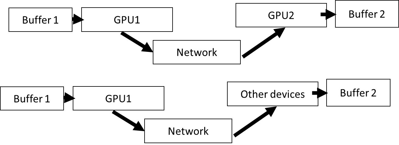
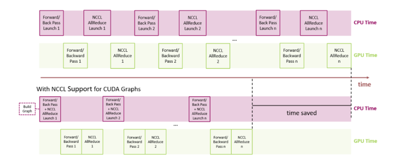
CPU and GPU communication has its own kernel (implemented in NCCL
but it is essentially memcpy and operations (reduction,
distribution))
The overhead of NCCL can be high with fast iterations
image-20251209215702725
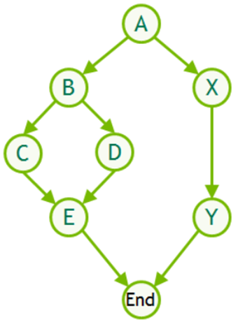
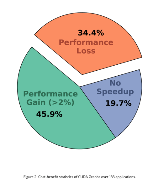
CUDA graph with Pytorch2
Is using CUDA graph always good?
The source of performance degradation
parameter value transfer (pointer to pointer operations)
The paper discuss CUDA graph-aware data placement
image-20251209215720273
What is the main advantage of using CUDA Graph?
A: To significantly reduce CPU overhead from repeatedly launching
many small kernels by capturing the whole GPU workload as a single
executable graph and replaying it efficiently.
Paper Readings
What kind of applications would get benefits from a large warp?
A: Apps with highly regular, SIMD-friendly, data-parallel workloads,
where all threads follow the same control flow and access memory in a
uniform pattern.
What is the main advantage of register file virtualization in
GPUs?
A:It allows the GPU to support more threads (higher occupancy) than
the physical register file would normally allow, improving latency
hiding and overall throughput.
Why is it hard to support virtual address translation for GPUs?
A:Because GPUs execute tens of thousands of threads in parallel, and
virtual address translation requires page table walks and TLB lookups.
Supporting this at GPU scale produces huge latency, high energy cost,
massive TLB pressure, and large hardware area overhead.
Which statement explains the meaning of Unified Virtual Memory (UVA)
better?
A: UVA provides a single unified virtual address space shared across
the host and all GPUs, allowing pointers to be meaningful across devices
without explicit address translation.
When does GPU memory oversubscription happen?
A: Oversubscription happens when a GPU uses Unified Memory (Managed
Memory) and the application allocates more memory than the physical GPU
memory capacity.
What are the main benefits of 2-level warp scheduling?
A:(1) Better latency hiding (2) Better resource utilization (3)
Higher fairness among warps / thread blocks (4) Improved energy
efficiency
GPU Simulation
Performance Modeling
Techniques
Cycle level simulation
Event driven simulation
Analytical Model
Sampling based techniques
Data based statistical/ML modeling
FPGA based emulation
Cycle Level Simulation
Commonly used in many architecture simulators
Typically, a global clock exists.
Each cycle, events, such as instruction fetch and decode are
modeled.
Trace-driven simulators are simpler and often lighter and easier
to develop
E.g.) Memory traces only for memory simulation or cache
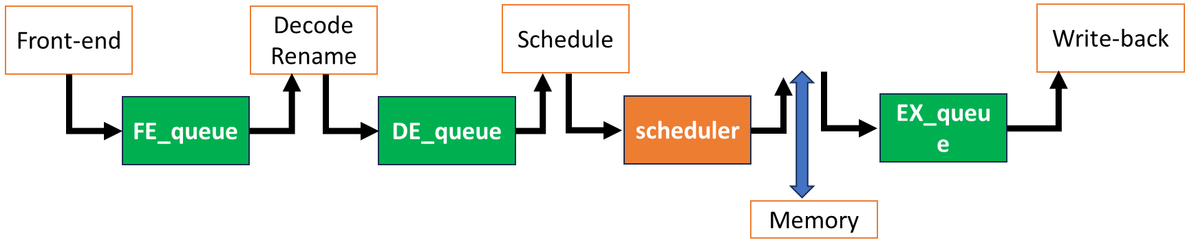
Queue Based Modeling
Instructions are moving between queues.
Scheduler selects instructions that will be sent to the execution
stage among ready instructions; not implemented as a queue
structure.
Other queues are FIFO.
When instruction is complete, the dependent instructions are
ready. The dependency chain needs to be modeled and broadcasting also
needs to be modeled.
Cache and memory are modeled to provide memory instruction
latency.
image-20251210002400840
Modeling
Parameters with Queue Based Modeling
Number of cycles in each pipeline stage → depth of the
queue
How many instructions can move between queues represent pipeline
width (E.g., Issue/execution bandwidth)
Questions: How do you know the latency of each
instruction?
Instruction latency assumptions:
Instruction latency is given as a parameter (e.g., ADD takes 1
cycle, MUL takes 3 cycles).
Latency can be obtained from literature or simulators like CACTI
or RTL simulation.
Scheduler chooses instructions from the head of each
warp.
Differences from CPUs:
In-order scheduling within a warp
Out-of-order across warps
Major differences between CPU vs. GPU
Handling divergent warps
Warp, thread block, and kernel concepts
Scheduler
End of Simulation
Entire thread block scheduled to one SM
Tracking complete threads
All threads within a cuda block, the corresponding cuda block
completes
When all thread block is completed, the kernel ends.
When all kernel ends, the application ends.
In the queue-based simulation, if we want to increase the execution
width, what change do we need to make? Please refer to the diagram in
the lecture for the module names. Choose the most relevant one?
A: the number of entries / parallel functional units in the Execute
stage
Which of the modules cannot be implemented with queue-based
modeling?
Mask bits are needed to keep track of resource
constraints.
Question: How to model divergent warps and memory
coalescing?
Memory Coalescing Modeling
Modeling memory coalescing is critical.
Memory requests need to be merged.
Typically, this follows cache line sizes.
A 64 B cache line size is already assumed.
Modeling Memory
Coalescing with Trace
The trace should contain all the memory addresses from each
warp.
The trace generator can insert all memory instructions
individually. E.g., va1, va2, va3, etc.
Or trace generator already coalesces memory requests → can reduce
the trace size: e.g.) 0x0, 0x4, 0x8, 0x12, 0x16 etc. vs. 0x0 and size
28
Cache Hierarchy Modeling
After addresses are coalesced, memory requests access TLB, L1, L2
caches depending on GPU microarchitecture.
Sectored Cache Modeling
Modern GPUs adopt sectored cache.
Sectored cache allows bringing a sector of the cache block
instead of the entire cache block.
Benefit: reduces bandwidth
Drawback: reduces spatial locality
Share the tag
GPU Simulators
Several open-source GPU simulators are available.
GPU simulators for different ISAs
Name
ISA
Type
Architecture
Open Source
GPGPU-Sim
NVIDIA PTX/SASS
Execution driven
GPGPU only
http://www.gpgpu-sim.org/
Accel-Sim
NVIDIA PTX/SASS
Trace driven
GPGPU and accelerator
https://accel-sim.github.io/
MGPU-Sim
AMD GPU
Execution driven
Multi GPUS are supported
[ISCA2019]
Macsim
NVIDIA/Intel GPU
Trace driven
Heterogeneous computing
https://github.com/gthparch/macsim
Gem5-GPGPU-Sim
AMD GPU or NVIDIA PTX
Execution driven
Heterogeneous computing
https://cpu-gpu-sim.ece.wisc.edu/
Vortex-Simx
RISC-V ISA (extensions)
Execution, RTL
3D graphics, GPU
https://vortex.cc.gatech.edu/
Which statement most accurately describes sectored cache and small
block size of cache?
A: Sectored cache reduces data transfer size while keeping a large
tag array;
small block size reduces miss penalty but does not reduce tag storage
overhead.
GPU Analytical Models
Analytical models do not require the execution of the entire
program.
Analytical models are typically simple and capture the first
order of performance modeling.
Analytical models often provide insights to understand
performance behavior.
First Order of GPU
Architecture Design
Let’s consider accelerating a vector dot product with a goal of 1T
vector dot products per second (sum +=x[i] *y[i] )
For compute units, we need to achieve 2T FLOPS operations (multiply
and ADD) or 1T FMA/sec.
If GPU operates at 1GHz, 1000 FMA units are needed; at 2GHz, 500 FMA
units are needed.
Memory units need to supply 2 memory bytes with a 2TB/sec memory
bandwidth.
500 FMA units are approximately equal to 16 warps (warp with 32).
If each SM can execute 1 warp per cycle at 2GHz and there are 16 SMs,
it can compute 1T vector dot products.
Alternatively, 8 SMs with 2 warps per cycle can also achieve
this.
Based on what we have discussed, if we want to design a processor for
1T vector dot products per second with a 4GHz GPU frequency, what’s the
memory bandwidth requirement?
A:
To have 1000 FMA units with a 32-thread width of warps, how many
warps need to be executed in one cycle with a 4GHz processor?
A:
Multithreading: How about the total number of active warps in
each SM?
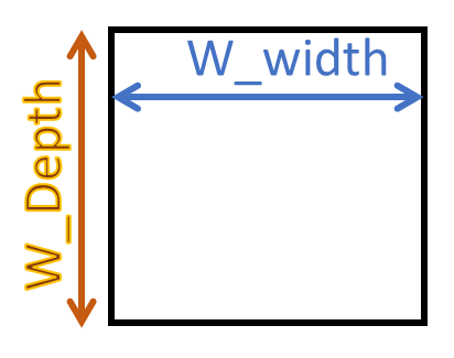
W_width : the number of threads (warps) that can run in one
cycle
W_depth: the number of threads (warps) that can be scheduled
during one stall cycle
W_depth and W_width H/W
Constraints
W_width is determined by the number of ALU units (along with the
width of the scheduler)
W_depth is determined by the number of registers (along with the
number of PC registers)
W_depth 20 means 20 x 32 (W_width) x (# register per thread)
number of registers are needed
W_depth 20 also means at least 20 x PC registers is
needed.
image-20251210005653933
Finding W_depth
Strong correlation factor of W_depth is memory latency.
In the dot product example, assume memory latency is 200
cycles.
Case 1) 1 comp, 1 memory (dot product):
To hide 200 cycles, 200/ (1 comp + 1 memory) = 100 warps are
needed
Case 2) If we have 1 memory instruction per 4 compute
instructions
To hide 200 cycles 200 / (1+4) = 40 warps are needed
Decision Factors for the
Number of SMs
Previous example: 500 FMA units
1 warp x 16 SMs vs. 2 warps x 8 SMs
Large and fewer SMs vs. small and many SMs
Cache and registers also need to be split.
Large cache with fewer SMs vs. small cache with many SMs
Large cache increases cache access time, but large cache can
increase cache hits among multiple CUDA blocks
Sub-core can also be a design decision factor
Many of these decisions require the analysis of trade-off between
size vs. time
What is most strongly correlated with deciding
W_width for the register file sizes
A:
The number of cores
The number of ALUs
The number of active threads
Memory latency
Roofline Model
image-20251210010949705
A Visual performance model to determine whether an application
(or a processor) is limited by the compute bandwidth or memory
bandwidth
Vector sum example: 2 Bytes per 1 FLOPS → arithmetic intensity :
0.5
Another example: sum +=x[i] x[i]y[i]*y[i]; → 2 Bytes per
4 FLOPS → arithmetic intensity: 2
CPI (Cycle per
Instruction) Computation
CPI = CPI + CPI + CPI +
CPU …
CPI: sustainable performance without any miss
events
Example: 5-stage in-order processor
Assumption: CPI = 1. CPI =3 ,
CPI = 5
2% instructions has branch misprediction. 5% instructions has cache
misses. Average CPI?
Answer: 1 + 0.023 + 0.055 = 1.31
Easy to compute the average performance.
All penalties are assumed to be serialized.
CPI Computation for
Multi-threading
CPI = CPI/W_depth
W_depth: the number of warps that can be scheduled during the
stall cycles
CPI = CPI + CPI
Resource contention: MSHR (# of memory misses), busy states of
execution units, DRAM bandwidth etc.
GPU is modeled for multi-threading
Applying Interval Analysis
on GPUs
Naïve approach: consider GPU as just a multi-threading
processor
Major performance differences between GPU and multi-threading
processor
Branch divergence: not all warps are active; some part of branch
code is serialized.
Memory divergence: memory latency can be significantly different
depending on memory is coalesced or uncoalesced
Newer models improve the performance models by modeling sub-core,
sectored cache, and other resource contentions more accurately.
Using the roofline model, we want to guide the performance
optimization directions. After plotting into the roofline model, it
turns out that the application is compute bounded. What would be a
better approach to improve the application?
A:
By utilizing shared memory, the amount of memory to bring is
reduced.
Check whether any of the compute operations can be
simplified.
Upgrade the GPU with more memory
Apply prefetching operations
A better approach is to reduce the amount of computation or increase
compute throughput, e.g., using a better algorithm (fewer FLOPs),
vectorization / tensor cores / lower precision, or other
instruction-level optimizations.
Accelerating Simulation
Accelerating simulation itself
Parallelizing the simulator
Event driven simulation
Simplifying the model
Sampling
Statistical Modeling
ML based Modeling
Reducing the workloads
Micro benchmarks
Reducing the workload size
Create small representative workloads
What techniques are the most helpful if we simulate Project #2’s
homework solution for GPU architecture simulation? Choose all apply.
Reduce iteration counts
Reduce input sizes
Identify dominant kernels and only simulate the dominant kernels.
__global__ voidassignClusters(constfloat *points, constfloat *centroids, int *assignments, int n_points, int k, int dim){ int idx = blockIdx.x * blockDim.x + threadIdx.x; if (idx < n_points) { int best_cluster = 0; float min_dist = FLT_MAX;
for (int c = 0; c < k; c++) { float dist = 0.0f; for (int d = 0; d < dim; d++) { float diff = points[idx * dim + d] - centroids[c * dim + d]; dist += diff * diff; // 1 FLOP multiply + 1 FLOP add per dimension }
The kernel is launched with enough threads to cover the condition
idx < N / 10.
Global memory is accessed in 128-byte aligned transactions.
There is no caching (every access results in a
memory transaction).
Memory bandwidth is measured based on data transferred from
memory to the core, including reads and writes.
Question: What is the approximate
floating-point operations per byte (FLOP/Byte) for this
kernel? Here we calculate Bytes for all the data that has to be brought
based on memory transaction sizes. (Choose the closest value based
on memory traffic, not just raw data accessed.)
A:
When counting bytes based on transaction size , each transaction transfers bytes and contains elements (E: bytes per element).
With a stride , only about of them are used. Thus, the
effective bytes per useful element is: For three arrays (two loads + one store), bytes per index is
, so the arithmetic intensity
is: In this kernel,
bytes, , hence FLOP/B.
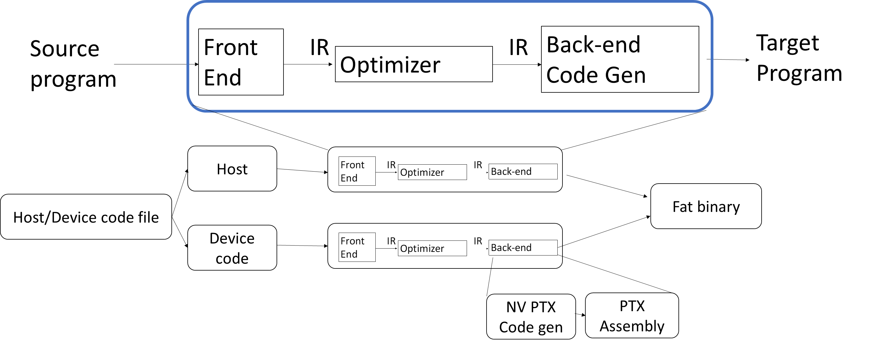
Compiler Intro
Compilation Flow
CPU Compilation Flow
image-20251210192317347
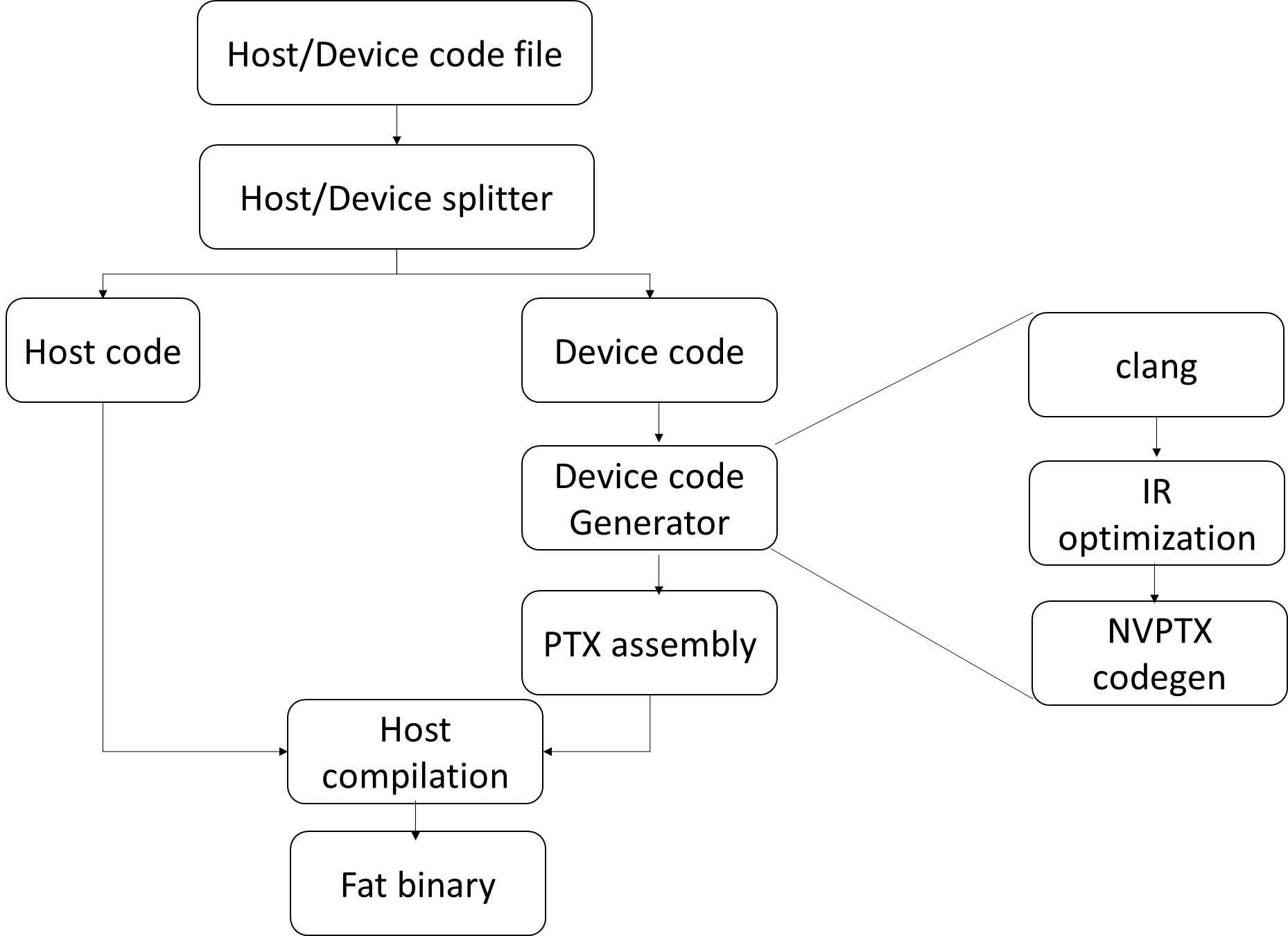
GPU Compilation Flow
image-20251210192344219
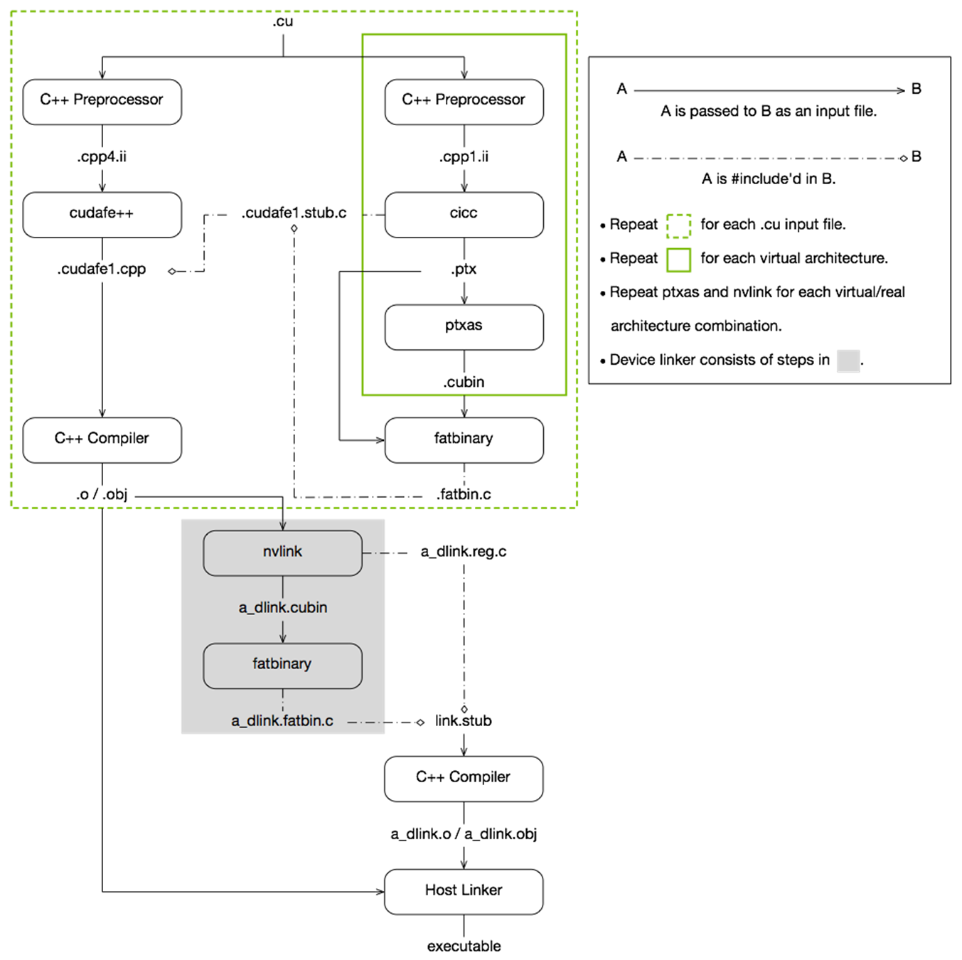
NVIDIA
image-20251210192525844
GPU Compiler Pass
image-20251210192616555
Roles of CLANG
Front end parser
Tool chain for C-family languages
Generating the Abstract Syntax Tree (AST)
C++ PreProcessor
Performs text substitution before compilation
1 2 3 4 5 6 7 8 9 10 11
#define COURSE_NUMBER 8803 Int main() { int number = COURSE_NUMBER; } // into
Int main() { int number = 8803; }
IR Optimizations
Intermediate Representation
Back-end compiler
IR provides a good abstract to optimize
Many compiler optimizations are done in the IR level
PTX vs. SASS
PTX
Parallel Thread Execution
PTX is a virtual ISA
Architecture independent
PTX will be translated to machine code
PTX does not have register allocation
SASS
Low-level assembly language
Shader Assembly
Architecture dependent assembly code
Register is allocated
Fat Binaries
It contains execution files for multiple architectures
It supports multiple GPU versions
It also includes CPU code
PTX Instruction
Zero to four operands
Optional predicate information following an @ symbol
A maximum sequence of instruction stream with one entry and one
exit
Only the first instruction can be reached from outside.
Once the program enters a basic block, all instructions inside
the basic block needs to be executed.
All execution needs to be consecutive.
Exit instruction is typically a control-flow
instruction.
Optimizations within a basic block are local code
optimization.
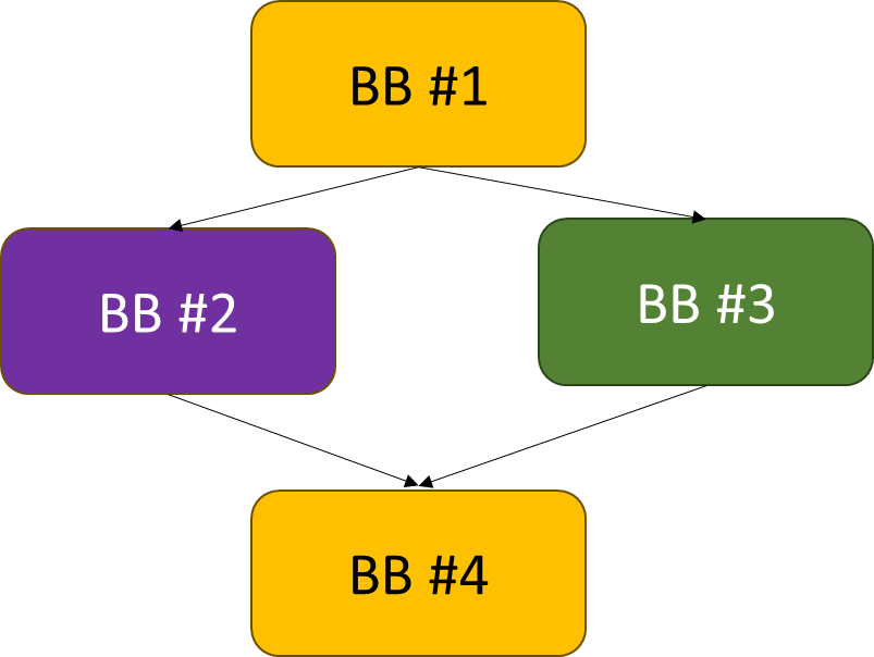
Flow Graph
Flow graph: each node represents a basic block, and path
indicates possible program execution path.
Entry node: the first statement of the program
1 2 3 4 5
If (cond1) // BB #1 do work1 // BB #2 else do work 3// BB #3 BB #4
image-20251210193919383
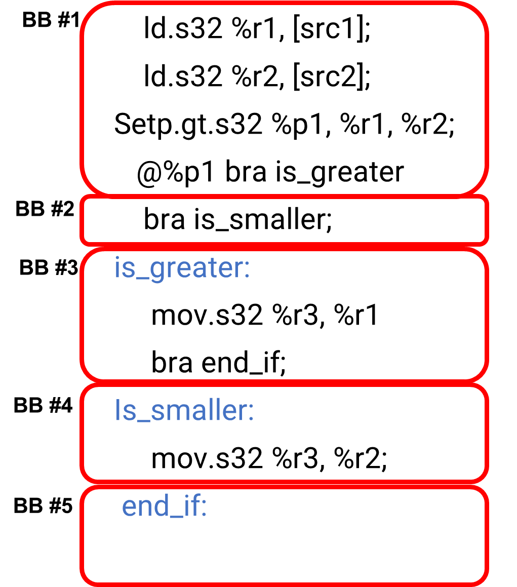
Example
1 2 3 4 5 6 7 8 9 10 11
ld.s32 %r1, [src1]; ld.s32 %r2, [src2]; setp.gt.s32 %p1, %r1, %r2; @%p1 bra is_greater; bra is_smaller; is_greater: mov.s32 %r3, %r1; bra end_if; Is_smaller: mov.s32 %r3, %r2; end_if:
Draw a basic block and Control Flow
A:
image-20251210194219243
Data Flow Analysis
Global Code Optimizations
Local code optimization: optimization within a
basic block
Global code optimization: optimization across
basic blocks
Most global code optimization is based on data-flow
analyses
Data-flow analysis:
Analyze the effect of each basic block
Analyses differ by examining properties
Principal sources of optimization
Compiler optimization must preserve the semantics
of the original program
Examples of Code
Optimizations
Removing redundant instructions
Copy propagation
Dead code eliminations
Code motion
Induction variable detection
Reduction strength
Data-Flow Analysis
Abstraction
Execution of a program: transformations of the program
state
Input state: program point before the
statement
Output state: program point after the
statement
Transfer Functions
Use Transfer Functions notation
OUT[B] = f_B(IN[B])
IN[B]: immediate before a basic block
OUT[B]: immediate after a basic block
: transfer function of
statement s
Predecessor of B: All blocks that are executed before the
basic block B
Successor of B: All blocks that are executed after the basic block of
B
Reaching Definitions
Analyze whether a definition reaches
A definition d reaches a point
p if there is a path from the point immediately
following d to p, without being killed
(overwritten)
Definitions: a variable is defined when it receives a
value
Use: when its value is read
E.g.) a= x + y → definitions: a, use: x, y
Gen and Kill
d: u = v + w
Generates the definition d of variable
u and kills all other definitions in the program that
define u. : the set of
definitions generated by the statement
: the set of all other
definitions of u in the program
Generalized Transfer
Functions
Reaching Definitions
Algorithm
1 2 3 4 5 6 7
OUT[ENTRY] = ∅ for (each basic block B other than ENTRY) OUT[B] = ∅ while (changes to any OUT occur) for (each basic block B other than ENTRY) { IN[B] = ∪_(𝑃 𝑎 𝑝𝑟𝑒𝑑𝑒𝑐𝑒𝑠𝑠𝑜𝑟 𝑜𝑓 𝐵 )OUT[P] OUT[B] = 𝑔𝑒𝑛_𝐵 ∪ (IN[B] - 𝑘𝑖𝑙𝑙_𝐵) }
image-20251210202247100
BB
Out[B]0
IN[B]1
OUT[B]1
IN[B]2
Out[B]2
B1
000 0000
000 0000
111 000
000 0000
111 0000
B2
000 0000
111 0000
001 1100
111 0111
001 1110
B3
000 0000
001 1100
000 1110
001 1110
000 1110
B4
000 0000
001 1110
001 0111
001 1110
001 0111
EXIT
000 0000
001 0111
001 0111
001 0111
001 0111
Live-variable Analysis
Live-Variable (Liveness)
Analysis
Liveness analysis helps determine which variables are live (in
use) at various program points.
Usage: register allocation. Register is allocated only for live
variables, ensuring registers are allocated only to live
variables.
Data-Flow Equations
: set of variables
defined in block B before any use
:"set of variables
whose values may be used in block B before any definition"
IN[EXIT] = ∅ : boundary condition
IN[B] =
OUT[B] =
Analysis is done in the backward (opposite to the control
flow)
Algorithm
1 2 3 4 5 6 7
IN[EXIT] = ∅ for (each basic block B other than EXIT) IN[B] = ∅ while (changes to any IN occur) for (each basic block B other than EXIT) { OUT[B] = ∪_(𝑠 𝑎 𝑠𝑢𝑐𝑐𝑒𝑠𝑠𝑜𝑟𝑜𝑓 𝐵 )IN[S] IN[B] = 〖𝑢𝑠𝑒〗_(𝐵 ) ∪ (OUT[B] - 〖𝑑𝑒𝑓〗_𝐵) }
Iterative process
image-20251210203157039
BB
First Pass
Second Pass
OUT[ENTRY]
m, n, u1,u2,u3
m, n, u1,u2,u3
IN[B1]
m,n,u1,u2,u3
m,n,u1,u2,u3
OUT[B1]
i,j,u2,u3
i,j, u2,u3
IN[B2]
i,j,u2,u3
i,j,u2,u3
OUT[B2]
u2,u3
j,u2,u3
IN[B3]
u2,u3
j,u2,u3
OUT[B3]
u3
j,u2,u3
IN[B4]
u3
j,u2, u3
OUT[B4]
∅
i, j, u2, u3
IN[EXIT]
∅
Register
Allocations and Live-Variable Analysis
image-20251210203745003
a is dead after BB #1
Register for a can be reused after BB
#1
b is still live at BB #2, if b is dead at BB #2,
the register for b can also be reused
Register Allocations
Only live variables need to have registers.
What if there aren’t enough registers available?
Register spill/fill operations to a stack
Values that won’t be used for a while are moved to the
stack.
PTX assumes infinite number of registers, so stack operations are
not explicitly shown.
SSA
SSA is an enhancement of the def-use chain.
Key feature: variables can be defined only once in SSA
form.
Common usage: Intermediate Representations (IR) in compilers are
typically in SSA form.
image-20251210204218924
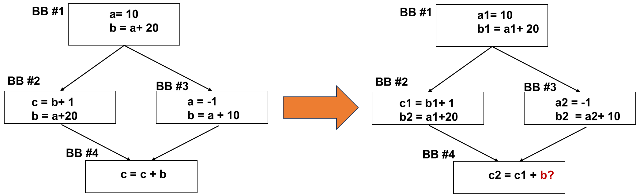
SSA and Control Flow Graphs
What if variable bs are defined in both places?
image-20251210204255961
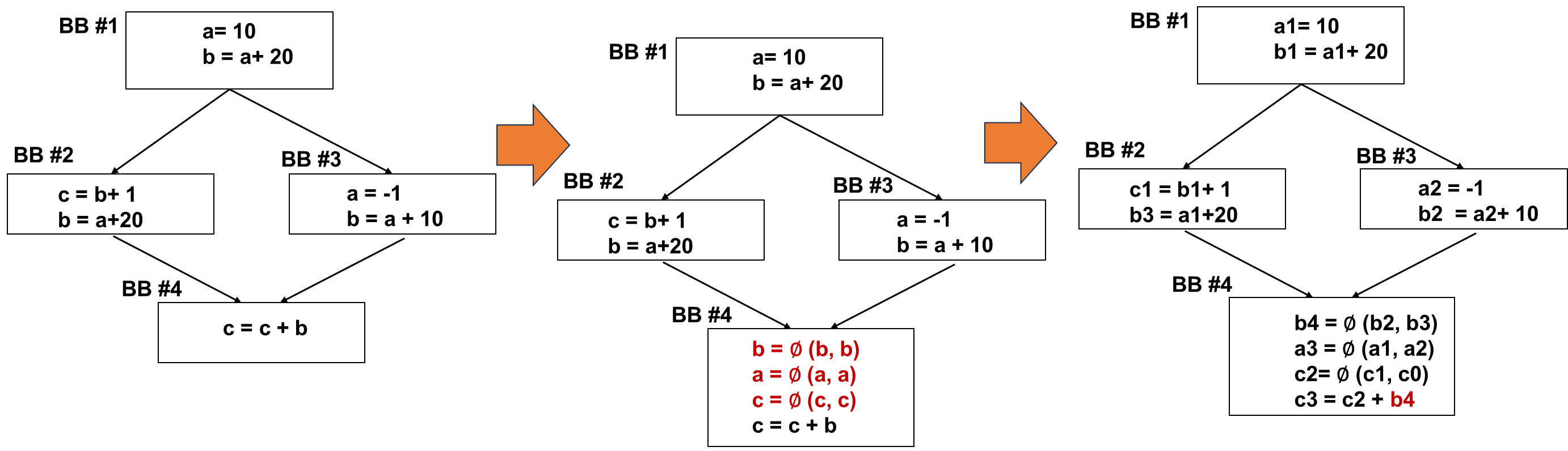
∅(𝑷𝒉𝒊)− Function
∅ Function merges values from different paths.
∅ Function can be implemented using move or other methods in the
ISA level.
Each definition gets a new version of the variable.
Usage always uses the latest version.
∅ Function is added at each joint point for every variable. →
more than one predecessor
SSA Conversion Example
image-20251210204355989
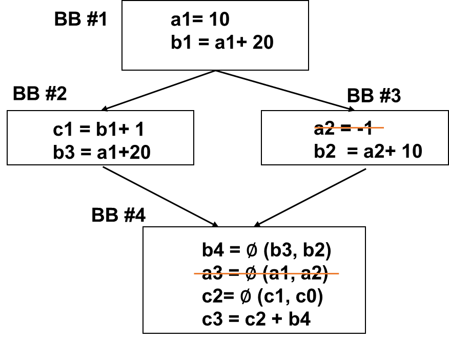
When to Insert ∅ Function ?
∅ Function is added at each joint point for every variable. →
more than one predecessor → can generate too many ∅ Functions
∅ Functions only need to be inserted when multiple values
exist.
image-20251210204457197
Iterative path-convergence criterion needs to be considered.
Path-Convergence Criterion
∅ Function needs to be inserted when all the following are
true:
1.There is a block x containing a definition of a;
2.There is a block y (with y x ) containing a definition of a;
3.There is a nonempty path P_xz of edges from x to z;
4.There is a nonempty path P_yz of edges from y to z;
5.Path P_xz and P_yz do not have any node in common other than z;
6.The node z does not appear within both P_xz and P_yz priori to the
end though it may appear in one or the other.
Initialization: start node has all variable definitions.
Examples of Compiler
Optimizations
Loop Unrolling
Unroll a loop for a small number of times for other code
optimizations
Benefits:
Better instruction scheduling
More opportunities for vectorizations
Reducing # of branches
1 2 3 4 5 6 7 8 9 10 11 12 13
for (i = 0; i <N; i++){ S(i); } //to for (i = 0; i+4 <N; i+=4){ S(i); S(i+1); S(i+2); S(i+3); } for ( ; i<N; i++) S(i); }
Detection: Identify loops with simple bounds and no non-affine
jumps or side effects.
Profitability Analysis: Estimate expected reduction in control
overhead versus potential increase in register pressure/code size using
heuristics and cost models.
Unroll Factor Selection: Choose unroll factor via static
heuristics, user-provided pragmas, or autotuning/profiling.
Transformation:
Expand loop body according to unroll factor.
Eliminate induction variable updates and conditional branches (when
possible).
Unrolling exposes opportunities to hold temporary
variables/arrays in registers by removing induction variables and index
computations.
Tradeoff: Large unroll factors increase register usage, reducing
occupancy (number of concurrent thread blocks).
Some compilers offer flags to restrict maximum register usage per
thread (e.g., --maxrregcount in NVCC).
Heuristic Pseudocode
1 2 3 4 5 6 7
for each loop L in kernel: trip_count = estimate_trip_count(L) max_unroll = hardware_limit() for unroll_factor in candidate_factors: profit = profile_simulate(L, unroll_factor) if profit > threshold and fits_in_register_file: apply_unroll(L, unroll_factor)
Branch-Divergence
Elimination: Code Example
1 2 3 4 5 6 7 8 9 10
if (condition) { x = a; } else { x = b; } //to x = condition ? a : b;
// Or, eliminating branch: x = a * cond + b * (1 - cond); // cond is 0/1
Compilers can convert eligible branches to predicated
instructions
Compiler
Algorithms for Branch Divergence Reduction
Control-Flow Analysis: flag likely divergent
branches.
Predication: replace simple branches with masked
ops.
Branch Flattening: merge/move branches;
1 2 3 4 5 6 7 8 9
for (int i = 0; i < N; ++i) { if (condition(i)) { // rare, complex path special_case(); } else { // common, fast path normal_case(); } }
1 2 3 4 5 6 7 8 9 10
for (int i = 0; i < N; ++i) { // common, fast path normal_case(); } if (condition(i)) { // rare, complex path undo normal case’s task special_case(); } else { }
Kernel/Loop Fission
1 2 3 4 5 6 7 8 9
for i = 0 to N-1 A[i] = B[i] * C1 C[i] = B[i] + C2 // up to down: loop fission // down to up: loop fusion for i = 0 to N-1 A[i] = B[i] * C1 for i = 0 to N-1 C[i] = B[i] + C2
GPU and ML
Why are GPUs Good for ML?
High number of floating-point operations
High data parallel operations
GPUs have dense floating-point operations
High memory bandwidth (e.g. GDDR, HBM)
Flexible data format standards (e.g. TF, BF, INT4 etc.)
Statistical computing based computations
DNN Operation Categories
Elementwise operations
E.g.) Activation operations
Reduction operations
E.g.) Pooling operations
Dot-product operations
E.g.) Convolution operations, GEMM
Background of GEMM
General Matrix Multiplications (GEMM)
C = α AB + βC
A, B and C are m x k , k x n and m x n matrix
α = 1 and β = 0 becomes C=AB
Popular in fully-connected layers, convolution layers
Production of A and B → M * N * K fused multiply-adds (FMAs) → 2
MN*K FLOPS
E.g.) FP 16 inputs FP32 accumulator
Arithmetic Intensity =(number of FLOPS )/(number of
bytes accesses ) =(2 (MNK))/(2(MK+NK+MN) )
Use Arithmetic intensity to compare the machine’s
FLOPS/B
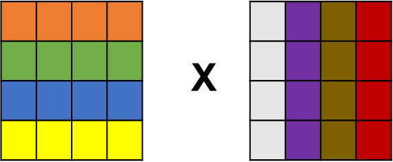
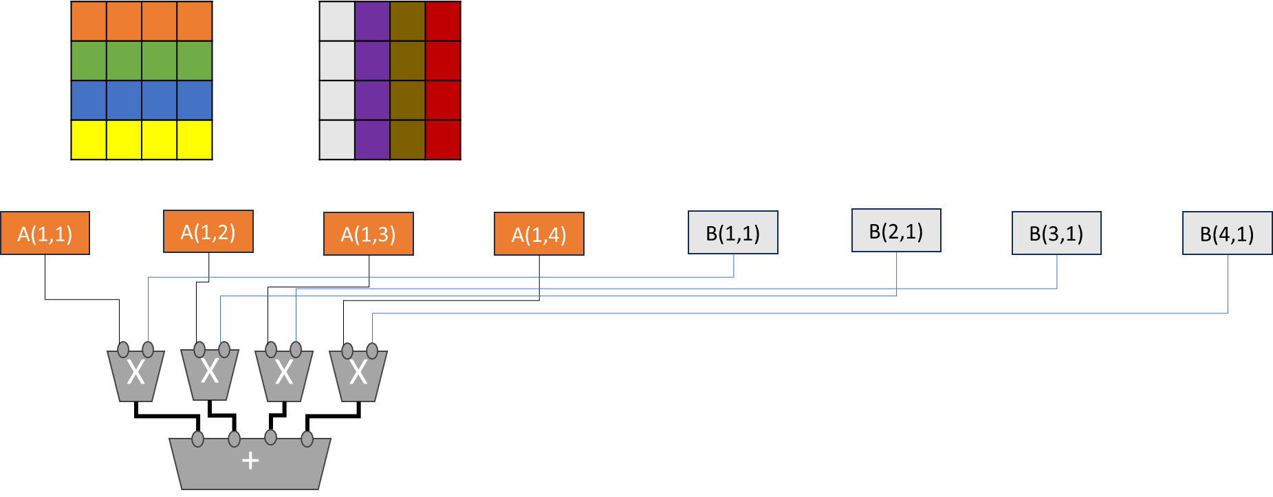
Difference Between SIMD vs.
Tensor
4x4 matrix computation
4 threads and each thread repeats a loop
image-20251210214359611
1 2 3 4 5 6
if (row < N && col < N)  {
    for (int i = 0; i < N; i++) {
      sum += A[row * N + i] * B[i * N + col];
   }
}
 C[row * N + col] = sum;
into
1
HMMA.1688.F16
Sum needs to be stored in a register. Since NVIDA thread is private,
one thread needs to perform accumulation.
If 16 threads are performing the work in parallel, the sum variable
needs a reduction mechanism.
SIMD/SIMT
Operations of Matrix Multiplications
- 16 SIMD/SIMT operations are needed for 4x4 matrix
multiplications.
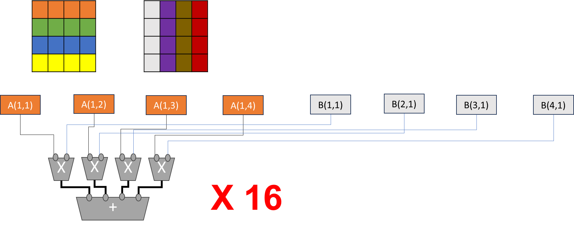
Tensor Cores
Tensor Cores perform matrix multiply and accumulate (MMA)
calculations.
Hundreds of Tensor Cores operating in parallel in one NVIDIA GPU
enable massive increases in throughput and efficiency.
Support sparsity
E.g.) Each A100 tensor core can execute 256 FP 16 FMA.
INT8, INT 4 and binary 1-bit predictions added
Transformer Engine
Introduced GH architecture
To accelerate transfer layers
Transformer engine dynamically scales tensor data into
representable range
FP 8 operations
Bring a chunk of data efficiently to fully utilize tensor
units
TMA address generation using copy descriptor
Floating Point Formats
FP 16 vs. FP 32
FP 16 uses the half precision of FP 32
IEEE standards have 32 bits/64 bits (singe/double
precisions)
Recap: Production of A and B à M * N * K fused multiply-adds (FMAs) à
2MN*K FLOPS
E.g.) FP 16 inputs FP32 accumulator If FP 8 inputs but FP32 accumulator Changing the input FP formats can change the arithmetic
intensity significantly.
Benefits of Quantization
Reduce the storage size
Increase the arithmetic intensity
Advanced floating-point operations also increase the
throughputs
E.g.) Ideal performance: the performance of FP 8 is 2 x of FP 16
operations
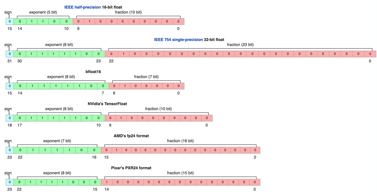
Different Floating Point
Formats
image-20251210215232979
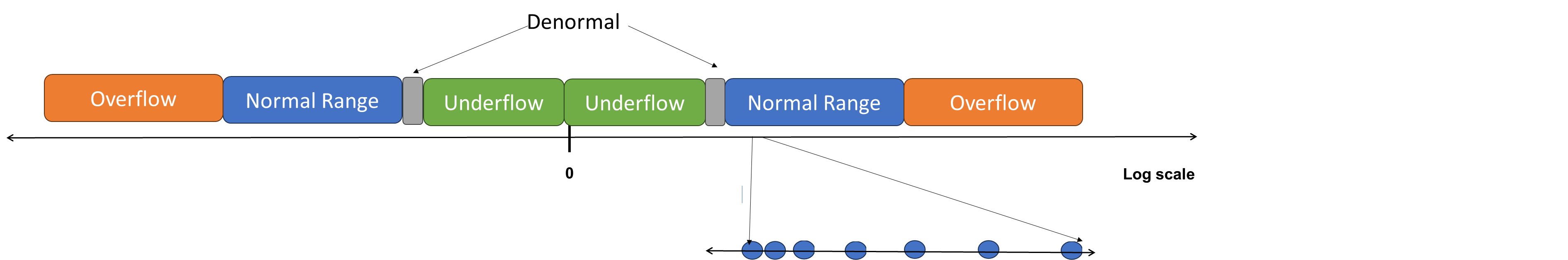
Some More Details
Exponent values can be both positive and negative
Floating points need to represent 2^(-exp1) to 2^(exp2)
Negative exponent values represent less than 1; positive exponent
values represent greater than 1.
Sign bit is to indicate negative or positive value of actual
floating point.
How to represent exponent values without sign bits?
Solution: offset the value
Subnormal numbers (denormalized numbers): when all exponents are
0
Floating Point Number
Representations
image-20251210215325227
Quantization
Reduce the number of required operations
Commonly used for reducing input operations while keeping the
accumulator in high precision
Quantization often leads to a non-uniform quantization
Sometimes, value transformations are used to overcome non-uniform
quantization.
E.g.) Shifted and squeezed 8-bit format (S2FP8)
Tensor Cores
Designing ML Accelerator
Units on GPUs
Consideration factors
What functionality?
Benefits over the existing GPUs
Compute unit design and the scale
Data storage and movement
Common Steps of
Designing Accelerators
Step 1. Identify frequently executed operations
Step 2. Performance benefit estimation
Software approach vs. hardware approach; software approach is
using the existing ISAs.
Step 3. Design interface and programmability
What ISA to add? What storages? Separate registers or shared
registers
Step 4. Consider to combine multiple features
Any other operations to combine?
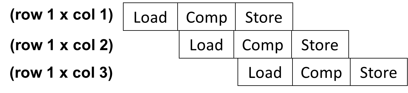
Matrix Multiplication
Accumulator
Mostly commonly used in ML workloads
SIMD operations still require row-by-row operations
Large matrix multiplication units can be implemented with
systolic arrays
Design decisions: many small matrix multiplication units vs. a
large matrix multiplication unit?
Area and programmability choices
NVIDIA started with 4x4x4 matrix multiplication units
Option 1: Parallel Units 4 FMA units x 16 elements
Option 2: Pipelining with future FMA units
image-20251210215725202
Data Storage and Movement
Input matrices have to come from Memory
Design decisions: dedicated registers or shared memory
4x4x4 matrix operations require at least 3 x 16 register
space.
NVIDA, registers are private to threads
Memory space can be used for storing tensor data.
Eventually, data needs to come from memory.
In NVIDIA, with tensor core, new asynchronous copy instruction is
introduced[1]: loads data directly from global memory into shared
memory, optionally bypassing L1 cache, and eliminating the need for
intermediate register file (RF) usage
New asynchronous barrier instructions are also
introduced.
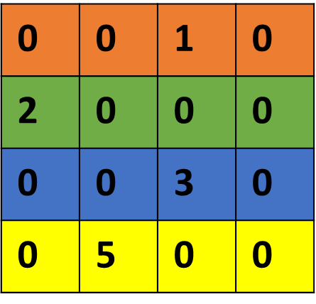
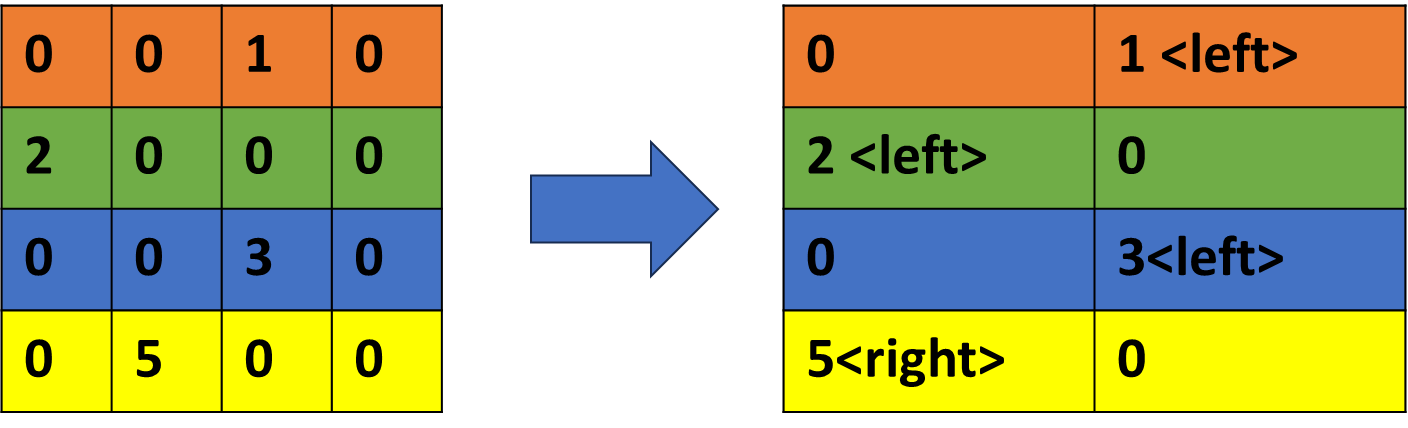
Supporting Sparse Operations
Sparse Matrix Multiplication: some elements are zero
values
Widely used in high-performance computing programs
Software approaches: use compressed data format
Instead of storing all values, only store non-zero
values
Structured sparsity: assume only a fixed % of elements are
non-zeros
E.g.) Assumption of 50% sparsity (use 1 bit to indicate left or
right position)
image-20251210215912903
With a structured sparsity, storing index information is
simplified.
Accelerating SpMV (Sparse Matrix-Vector Multiplication) is a big
research topic.
Reduce storage space and throughputs
Exam Practices
In the queue-based simulation, if we want to increase the execution
width, what change do we need to make? Please refer to the diagram in
the lecture for the module names. Choose the most relevant one?
A. Increase the width of DE queue
B. Increase the width of FE queue
C. Increase the depth of DE queue
D. Increase the number of ops to select in the
scheduler
Option
Why it's NOT the right one
Increase the width of DE queue
DE queue stores decoded ops; wider queue doesn't change how many
execute per cycle.
Increase the width of FE queue
Same reason, FE queue affects fetch bandwidth, not execution
width.
Increase the depth of DE queue
Depth = how many ops it can hold, not how many can issue per
cycle.
Which statement most accurately describes sectored cache and small
block size of cache?
Sectored cache is good for reducing cache size.
Sectored cache and small cache block size could reduce the
memory bandwidth requirements.
Sectored cache is good for improving spatial locality.
Both sectored cache and small cache block size have the same cache
tag storage requirements.
✘ Sectored
cache is good for reducing cache size.
Wrong. Sectored cache mainly reduces tag storage,
not total cache size.
The data array size stays the same.
✘
Sectored cache is good for improving spatial locality.
No. It actually helps when spatial locality is
poor, since you don't want to fetch the whole block.
Spatial locality improvement comes from large blocks, not
sectored design.
✘
Both sectored cache and small cache block size have the same cache
tag storage requirements.
Also false.
Sectored cache: 1 tag per large block.
Small block size cache: 1 tag per small block →
many more tags → higher tag storage.
Assuming 100 CUDA blocks, each consisting of 100 threads, with a warp
width of 16, and a page size of 4KB, what optimizations would be most
helpful in reducing address translation overhead in this code? The
baseline machines has 16 entry L1 TLB per core and 48 entries for L2 TLB
which are shared among all the SMs, and there are 4 SMs. One SM can
execute one CUDA block at a time. L1 TLB access time is 1 cycles and L2
TLB access time is 10 cycles. Float uses 4B.
Double L1 TLB size
Double L2 TLB size
Doubling L1 TLB or Doubling L2 TLB will have similiar performance
improvements
Doubling L1 TLB or Doubling L2 TLB will not show any
benefits.
A: enough L1 for now
Which analysis is good for dead code eliminations?
Liveness analysis
Strength Reduction
Constant Propagation
We want to the draw roofline graph. This is measured data from A100
and H100
Question 3 From the above measured data, find the peak compute
throughput for A100 Choose the closet number. Assume that measured data
reach the compute bounded zone. A100: 5000GFlop/s A100:
1TFlop/s A100: 10TFlop/s A100: 100TFlop/s
A:
BW=0.166667228.428=1370.6 GB/s
BW=0.166667466.77=2800.6 GB/s
(use lowest datapoint)
We want to represent the following decimal numbers in binary
floating-point format:
(1, 1.2, 0.75, 1.1, 0.2, 0.1)
Which of the following is the best choice for mantissa and exponent
format to represent these numbers with reasonable precision?
Question 2 ou are performing a 4×4 × 4×4 matrix multiplication using
vector operations on a machine with vector registers of width 4. The
machine can perform 16 vector operations simultaneously (i.e., SIMD
parallelism across 16 vector instructions).
What is the minimum number of vector registers required to hold all
intermediate data during the computation?
8 12 16 24
A: 4(A) + 4(B) + 4(C) + 4(temp register)=16
Question 3 1 / 1 pts You are performing a 4×4 × 4×4 matrix
multiplication using tensor operations on a machine where:
Each vector register holds 4 floating-point values, The tensor core
can compute the entire 4×4 × 4×4 multiplication in one fused operation.
What is the minimum number of vector registers required to hold all
input and output data for the computation? Partial sums that are stored
in the tensor units are not counted.
12 16 20 24
A: 4+4+4=12
[GPU-design-part-a]
You are designing a GPU system that should fully utilize the
available memory bandwidth.
Here are the system details:
The memory system is HBM with a peak bandwidth of
3 TB/s.
The data format used is BF16 (bfloat16), which is
2 bytes per value.
Each operation is a Fused Multiply-Add (FMA) that
uses 2 input values and produces 1 output, meaning
3 memory accesses per operation.
Each Streaming Multiprocessor (SM) runs at
1 GHz and can execute 2 warps per
cycle.
Each warp has 32 threads, and
each thread performs 1 FMA per cycle.
Assume there is no cache, and all memory accesses
go directly to HBM.
What is the minimum number of SMs needed to fully
saturate the 3 TB/s memory bandwidth?
A:
3TB/s ->
1SM ->
Option: A. 5 B. 25
Choose A since we need fully
utilize resources
[GPU-design-part-b]
Now let's continue from the previous setup.
Assume all system parameters are the same as in
[GPU-design-part-a], except the
following change:
The GPU system now includes a cache with a
90% hit rate, meaning that only 10% of
the memory accesses go to the HBM.
With this 90% cache hit rate, what is the minimum number of
SMs needed to fully saturate the 3 TB/s HBM
bandwidth?