cs8803 Procedural Content Generation

2025-12-11 总结 0 评论

0821

Transformation

Scale

scale by

Translate

Translate by :

Rotate

Order matters

Rotate first, translate later ≠ Translate first, rotate later

Can group objects into hierarchies - objects make of sub-path

Visible object in Unity: Unity Objects

Create parent: make empty object, drag child under parent

Each object has its own transformatios.

Hierarchy window

(world)
	head
		face
		hat
			brim
			hat top

Read transformation from botton to top. (Scale Rotate Translate)

Scene View - edit object

Hierarchy - shows all game objects

Inspector - shows the components of objects:

Components

transformation
mesh filter
mesh render
collider
script-code,C#

Project - items in the assets folder

Assets

material
Texture
Meshes

Triangle

Grapic cards (GPU's) are made to draw triangles

Why?

Fit sized memory footprint. Alway planar.

vertex- vertices

Triangle/polygon face

Can buid complex shape with lots triangles.

Unity uese indexed face sets to storce meshes.

Indexed Face Set - list of vertices, list of face that reference

Tetrahedron

Index	Vertices
0	(1,0,0)
1	(0,1,0)
2	(0,0,1)
3	(1,1,0)

order vertices clockwise when viewed from outside

Faces
1,0,2
1,3,0
1,2,3
0,3,2

Create Mesh

1 2	Mesh my_mesh = new Mesh() g_obj.getCompoenet<MeshFilter>().mesh = my.mesh;

Make Vertex List

Vector3[] verts = new Vector3[4]; // 4 for vertices number
verts[0] = new Vector3(1,0,0);
verts[1] = new Vector3(0,1,0);
...

Vector3 - 3 floats

Make Faces

1
2
3

int[] tris = new int[12]; // 3x number of triagle
tris[0] = 1; tris[1] = 0; tris[2] = 2; // 1st triangle
tris[3] = 1; ...

Diffuse Surfaces

not shiny (e.g. paper, matte print, chalk)

normal - unit vertex perpendicular to surface

brightness of surface prependicular to

if is unique length, then

0826

1	my_mesh.RecaculateNormal();

For sharper look - do not smooth a mesh's adjacent normals by averaging them

Random Numbers - at the heart of PCG

let use credic variations in a scene

In graphics of games: use pseudo-random numbers

not strictly random
use predictable, sophisticated algorithms
can generate random numbers in a predictiable way (random seed)

Use of random numbers

select from distint options (e.g. brick vs. wood house)
placement of objects (e.g. trees in forest or park)
parameter
- height of dinosors
- color of fish(red, grenn, blue)

Assuem: random routine random() <- returns float in [0,1)

get integer between 0 and n-1

1	rand_int = (int) floor(random()* n);

Random number seed

let us repeat random sequences

create sequences from one seed
Minecraft + No Man's Sky
Seed are usually integers

Random routine: seed(s); "s" is an integer seed

seed(12);
print(random());	//0.1348
print(random());  //0.7225
seed(12);
print(random());	//0.1348
print(random());  //0.7225
seed(13);
print(random());  //0.6565

Ex.

if (random()<0.3)
	do_this();	//30% chance
else
	do_this();	//70%chance

int pick = (int)floor(random()*4);	// 0 to 3
Switch(pick) {
	case 0: xxxxx; break;
	case 1: xxxxx; break;
	case 2: xxxxx; break;
	case 3: xxxxx; break;
}

Random color

1 2	color c = new Color(random, random(), random(), 1.0f); //read green blue apacity, alpha

Random point in square

for (int i=0;i<20;i++){
	float x = random();
	float y = random();
	draw_point(x,y);
}

Random point in circle : rejection sampling

pick random point in square
reject point if not in circle ()

Random point on circle or sphere

generate random point in circle
project to surface of circle

1
2
3

float len = sqrt(x*x+y*y);	//assue circle center is (0,0)
x/=len;
y/=len;

random() gives equal probability of any number

probablity density function

sometimes we want some values to be more likely:

1 2	float r =random(); r=r*r;

vehicles often require paths

cars/streets
trains/tracks
wagon/dirt road
gondola/canal
hikers/trails

Streets of cars popular in games

sim city
City: Skyline
Grand Theft Auto
Large City Undercover
Super Mario Kart

How to make strees

real stress: OSM Open Street Map
fictional cities: use PcG!

Two approaches:

Grid-based(today & Thursday)
free-form(later)

0828

Method2 Recursive Subdivision

create binary (or grid) tree of region
each reigon has min&max x,y ranges

Montains can be ragged(Rockies) or smooth(Appalachians)

What to make: height field

Height field: 2D array of height of each all the array

Can render this as a 3D polymon mesh (tirangle or suqare)

Note: cannote give caves or overheads

Create terrain height values？

Random numbers！(Noise)

Maintain can be rugged or smooth

We want to control the randomness

Noise: white, band limited, fractal(1/f), blue...

White noise

Every is random & independent of neighbors.

Ex: static image on an old TV

Band-Limited Noise

Controlled randomness

Some corellation between nearby values.

No coreletion between far apart locations.

1D value noise(smooth join of random values)

Not great:(too much low of frequencies) can have long stretches that are nearly the same in value

1D Perlin noise(band-limited)

Ken Perlin

Mkae function go up and down regularly

Use slope instead of values

Smooth: No overly large similar height

Actually do this in 2D or 3D

Want: repeatablity of values - same result that start them

Use: random number seeds

float noise1d(float x){
  int P1=floor(x);
  int P2=floor(x)+1;
  float t = x-p1;
  random_seed(P1); slope1 = random_int(2)*2-1;	//1 or -1
  random_seed(P2); slope2 = random_int(2)*2-1;
  return  (smooth_interp(slope1, slope2, t));
}

2D * 3D noise is similar

interp in (x,y) or (x,y,z)

Perlin noise can give smooth hills. Rough mountain?

high amplitude low fre = 1/wavelength
Mid. amp. mid freq.
low freq. high freq.

0902

Mazes

Many video games mazes

central to game(PacMan)
as mini-puzzles
parts of dungeon creation

Early mazes had paths that were not branched (unicursal)

Junctions(branches) were added. Most basic form is simply connected

Can solve by putting hand on one wall.

Multiply-connected maze

(Islands)

hand-on wall will not always solve!

Start with many isolated cells. Then knock down walls.

Only knock out walls that connect separate region.

Tracking regions

Classic group algorithm problem

Early but slow:

Overwrite number in one cell with the other of the cell if is joined to.

Two approaches to randomly deleting walls

Brute force: randomly pick a wall, see if it's not yet deleted(slow at end)
create list of all walls, select from this, update list

Faster way to determine connected regions

union-find(disjoint sets)- data structure & algorithm

High-level description

each region has one "root" cell
All other cells in conncected region point(maybe indirectly) to root(→)
Union(connect) two regions, cause one regions's root to make it point to the other region's root
pointers along the way are updated to take shorter path to root

Each union operation is nearly constant time. (inverse Ackerman function)

Many variations possible

delete more edges than you need: islands

can use other cell shapes: e.g. hexagons

can arrange cells in circles

Dungeons in Games

Role Playing Games(RPG)
Adventure-style (puzzle)
Hack& Slash(combat)
Roughe-like

Key fatures of dungeon layouts

multiple connected rooms or caverns
all rooms reachable
rooms can vary in szie or shape
many include doors (exp. in puzzle games)

Major Theme: room connectivity

Many was to create dungeons.

Tile Based Approach to Dungeons

similar to maze creation

Usually square cells.

0 - Wall

1 - no wall

2 - door in wall

All small Roooms

Run maze creation algorithm, gives fully connected sets of cells.

Big to Small Rooms (0 - wall, 1 - no wall, 2 - door in wall)

Randomly plaze large rooms in grid. Don't overlap rooms.
Use a maze-generation algorithm on the remaining open space to create hallways that connect the rooms.
Clean up the hallways and add details like doors and decorations to finalize the dungeon layout.

Big Room & Hallways

Place big room in grid, but not touching

Un-marked walls are hallways.

Knock-out doors: 0

Cellular Automata

Rules for changing grid cell states

Game of Life

09/04 — Streets (Free Form)

1. Overview

Free-form street generation aims to produce road networks that follow natural urban evolution rather than a rigid grid pattern.
Procedural algorithms must balance connectivity, realism, and terrain adaptation, while allowing parameters to control style (organic, radial, grid-like).

Traditional grid methods fail to capture historical or topographic influences; free-form methods simulate how streets grow under local and global constraints.

2. Street Generation Models

2.1 Agent-Based Growth Models

Each active street endpoint is treated as an agent with local rules.
At each time step, an agent can extend, branch, or terminate based on environmental cues.

Typical local rules:

Continue forward unless a collision or boundary is reached.
Branch with probability .
Avoid collisions by steering around nearby segments.
Stop if within threshold distance from existing roads.

Pseudocode

for agent in active_agents:
    dir = agent.direction
    new_pos = agent.pos + step * dir
    if too_close_to_road(new_pos): 
        agent.stop()
    elif random() < p_branch:
        spawn_agent(agent.pos, rotated(dir, θ))
    else:
        agent.pos = new_pos

This approach produces organic, branching patterns that resemble historical street layouts.

2.2 Tensor Field Method

Introduced by Parish and Müller (2001), this approach defines a tensor field over the terrain to represent desired street orientations.

A tensor field encodes a symmetric matrix describing the local preferred directions:

The dominant eigenvector of defines the principal direction for road growth.

Street agents integrate along the field:

This ensures global directional coherence (e.g., radial from city center or aligned to terrain slope).

Tensor fields are often generated by blending:

2.3 Potential Field Approach

A scalar potential field defines attractive or repulsive zones:

Low potential → desirable (downtown core)
High potential → undesirable (rivers, obstacles)

Agents follow the gradient descent:

The potential is often constructed as a weighted sum of population density and obstacle penalties: where is population density, is obstacle cost.

2.4 Combined Multi-Field Model

Modern systems combine both tensor and potential influences: This coupling allows streets to follow overall orientation while adapting to local density and constraints.

3. Connectivity Control

To prevent disconnected fragments, intersection detection and merging are performed:

Intersection test: if distance between endpoints < threshold, merge.
Angular snapping: adjust orientation to align to nearest road within .
Hierarchical merging: major roads first, local roads later.

4. Parameter Control

Parameter	Meaning	Typical Range
	branching probability	0.05–0.25
	min intersection distance	2–10 m
	branch angle	15–45°
	tensor vs potential weights	0.3–0.7
step	agent growth step size	1–10 m

5. Evaluation Criteria

Connectivity: single connected network.
Coverage: proportion of domain covered by roads.
Curvature smoothness: low average angular change.
Adaptation: roads follow elevation contours and avoid obstacles.
Hierarchy: differentiation between major and minor roads.

6. Exam Focus

Explain how tensor and potential fields guide road growth.
Compare agent-based, tensor field, and potential field models.
Derive how defines local orientation.
Describe how merging and snapping ensure connectivity.
Discuss trade-offs between local stochasticity and global coherence.

0909

Erosion

Natural terrain creation:

landmass creation(uplift)
erosion

New landmass creation:

Volcanism(e.g. Hawaii)
motion of tectonic plates (Appalachia)

Erosion

Termal(material knocked loose, piles up below)
wind
Glacier
Hydronic

"The Synthesis and Rendering of Eroded Fractal Terrains"

Siggraph 1989

Hydraulic erosion simulation steps

create fractal height field (e.g. Perlin noise) on aa square grid
deposit water at random locations(rain)
waterflow downhill
fast moving water picks up sediment
slow water deposit sediment

Each vertex has info:

altitude of terrain ()
water amount ()
sediment in swater ()

Each vertex may move water to four neighbors

Consider vertex v and geighboring verrtex u:

Amount of water paasted from v to u if

t = current time

t+1 = next time step maybe pick up sediment in

K_d = how fast sediment can be deposited

K_c = how much sediment water can carry

K_s = how easy is it for water to pickup soil(soil surface)

Repeatedly move water of soil over time steps t, t+1, t+2, ...

Result

Water carves channel in terrain
sediment picked up an steep slope(up high)
sediment deposited in flat areas(blow)

Snowball Algorithm (Job Talle)

move vertex along one path at at a time

place random ball on terrain
it rolls downhill
picks up sediment if moving fast
deposits sediment if slow
repeat this many times

Random Distribution

PDF (Pobability Density Function)

1
2
3

r = random();
x = r*r;
y = random();

Ken Perlin calls this bias.

Christoph Schlick's version

bias(r, .25) opposite to Bias(r, .75)

bias(r, .5) same to random() Like brightless control of screen

Can also control contract. (Pushed values towards or away from .5)

Called gain.

Gain function in 2 bias curves stifched together Can modify distributions by combing different random numbers.

r2 = (random()+random())/2.0;

Produce this PDF: peak at 0.5, triangle

R3 = (random()+random()+random())/3.0

Approach the Normal Distribution

Central Limit Theorem

Conbine several distribution

1 2	wsum = w1+ w2 + w3 conbine = (w1r1+w2r2+w3 +r3)/wsum

Ex. w1 = .8 w2= .2 w3 =0

09/11 — Building Facades

1. Overview

Facade generation defines the surface layout of architectural elements — windows, doors, balconies — after the building mass has been determined.
It is a hierarchical, grammar-based process that ensures style coherence and realism.

2. Hierarchical Decomposition

A facade is decomposed recursively into smaller structural units:

Each level applies split rules along horizontal or vertical axes.

Example:

1 2	split(Y) { 0.1:Base \| 0.8:MiddleFloors \| 0.1:Roof } split(X) { 0.1:Wall \| 0.8:WindowSection \| 0.1:Wall }

This yields a consistent floor and window arrangement.

3. Grammar Structure

3.1 Split Rules

Divide a shape along an axis:

3.2 Repeat Rules

Repeat elements across the facade with spacing control:

1	repeat(X, step=windowWidth){ Window \| Column }

3.3 Attribute Matching

Each shape carries attributes inherited and updated through rule expansion.
When selecting rules, matching ensures coherence between neighboring regions (e.g., same window size across one floor).

4. Parametric Facade Control

4.1 Geometric Parameters

Floor height
Window aspect ratio
Wall-to-window ratio
Balustrade height

These control realism and are sampled from architectural distributions.

4.2 Style Attributes

Materials, frame styles, and ornamentation are chosen probabilistically within style clusters: where measures style energy or deviation from theme.

5. Coherence and Symmetry

5.1 Vertical Coherence

Ensure balconies and window columns align vertically:

5.2 Horizontal Coherence

Ensure repetition of window style within each floor:

Symmetry constraints are commonly applied:

Mirroring left/right facade halves.
Pattern repetition every floors.

6. Detail Level and LOD

Facades can be represented with progressive detail:

Texture-based representation: distant view.
Procedural geometry: mid-range.
Full 3D components: close-up, for window frames and ornamentation.

Transition rules maintain consistency across LODs.

7. Pseudocode Example

def derive_facade(shape):
    if shape.label == "Building":
        split_y(shape, [0.1, 0.8, 0.1], ["Base", "Middle", "Roof"])
    elif shape.label == "Middle":
        repeat_x(shape, window_width, "WindowSection")
    elif shape.label == "WindowSection":
        attach_window(shape, random_style())

8. Randomness and Style Control

Procedural variation is introduced through stochastic rule selection while maintaining constraints.

Controlled randomness: where controls noise intensity on window sizes or spacing.

9. Exam Focus

Write a hierarchical grammar for a three-floor facade.
Derive and explain attribute matching.
Describe vertical and horizontal coherence constraints.
Compare deterministic vs stochastic rule application.
Explain multi-level LOD representation for facades.

09/16 — Building Shapes

1. Overview

Building shape generation defines the 3D volumetric structure of architecture before facade detailing.
The goal is to create plausible, style-consistent building masses that fit within urban and functional constraints.
This process extends from the principles of shape grammars and procedural modeling introduced by Müller et al. (2006, Instant Architecture).

2. Procedural Building Modeling

2.1 Shape Grammar Framework

A shape grammar defines rewriting rules that transform abstract shapes into more detailed geometry.
A rule has the form: where is a nonterminal shape symbol, and is an operator that splits, extrudes, or otherwise modifies the geometry.

Each building starts from a lot footprint and expands vertically using extrusion and subdivision rules.

Example

Building → Extrude(height=h) → Mass
Mass → Split(Y){ Base | Floors | Roof }
Floors → Repeat(Y, floorHeight){ Floor }
Floor → Split(X){ Left | Center | Right }

3. Core Geometric Operations

Operation	Symbol	Description
`extrude(h)`	⬆️	Raises a 2D footprint into 3D volume.
`split(axis)`		Divides a shape along an axis into parts.
`repeat(axis, step)`		Repeats a shape periodically.
`taper(angle)`		Applies linear scale gradient along height.
`roof(shape)`		Replaces top with a parametric roof (flat, gable, dome).

Operators can be deterministic (fixed size) or stochastic (sampled parameters).

4. Control Attributes

Procedural building models use attributes to control style and constraints:

Attribute	Symbol	Example
Height		sampled from normal distribution
Aspect ratio		defines building footprint proportion
Style		affects roof type and ornamentation
Symmetry		Boolean controlling mirrored parts

5. Roof and Volume Modeling

5.1 Roof Parametrization

Common roof types are defined by parameter sets controlling pitch and overhang:

Roof Type	Equation
Flat
Gable
Hip
Dome

5.2 Aggregated Structures

Complex buildings are created via CSG (Constructive Solid Geometry) union of sub-volumes: Each can be a procedural tower, base, or wing.
Hierarchical merging ensures topological consistency and stylistic coherence.

6. Shape Grammars and Instancing

Each rule produces geometry instances. Random seed and style weights define variation.

Example instancing rule:

1
2
3

split(X){ 0.4:Tower | 0.6:Wing }
Tower → Extrude(50)
Wing → Extrude(30)

This probabilistically generates towers or wings with different proportions.

7. Semantic Constraints

Procedural generation respects functional and physical constraints:

Lot coverage:
Height limit:
Sunlight constraint: maintain minimal setback to prevent shadow occlusion.

Violations are penalized via energy function:

8. Example: Pseudocode Implementation

def generate_building(lot, params):
    mass = extrude(lot, params.height)
    base, floors, roof = split_y(mass, [0.1, 0.8, 0.1])
    for i in range(params.n_floors):
        floor = duplicate(floors)
        apply_windows(floor)
    apply_roof(roof, params.roof_type)
    return combine(base, floors, roof)

9. Exam Focus

Write a shape grammar that produces a 3D building mass with variable roof type.
Explain difference between deterministic and stochastic subdivision.
Describe the role of attributes (height, style, symmetry).
Explain how energy constraints maintain realism.
Derive formula for gable/hip roof geometry.

09/18 — Tree Geometry

1. Overview

Procedural tree modeling captures the hierarchical branching structure of natural trees.
It combines biological rules (botanical structure) and algorithmic models (L-systems, self-organizing tree models).

2. Botanical Framework

2.1 Modular Units

Each tree is built from phytomers, repeated growth modules consisting of:

Internode (stem segment)
Leaf
Axillary bud (potential branch)

A branch can be recursively defined as:

2.2 Axis Hierarchy

Tree axes are categorized by order:

Order	Description
0	Trunk
1	Primary branches
2	Secondary branches
n	Higher-order twigs

Branch order determines scaling factors for length and radius.

3. Geometric Relations

3.1 Allometric Scaling

Empirical relationships govern branch geometry: where control geometric tapering.

3.2 Leonardo’s Rule

The sum of cross-sectional areas of daughter branches equals that of the parent: ensuring volumetric conservation across bifurcations.

4. L-System Models

A Lindenmayer system (L-system) defines string rewriting rules to model growth.

Example Grammar

1
2
3

Axiom: F
Rules:
F → F[+F]F[-F]F

Interpretation:

F = draw forward
+ / - = yaw rotation
[ / ] = push/pop turtle state (branching)

This recursive expansion produces a fractal-like branching tree.

5. Self-Organizing Tree Models (SOTM)

Introduced by Runions et al. (2007), these models simulate growth influenced by attraction points (light or nutrients).

Algorithm outline:

Scatter attraction points in space.
For each branch tip, find nearest attraction points.
Grow toward their centroid.
Remove points within influence radius .
Repeat until convergence.

Mathematically, new direction:

This produces natural, phototropically distributed branching.

6. Parameter Control

Parameter	Effect	Range
Branching angle	controls openness	20–60°
Tropism vector	global bias (e.g., toward light)	normalized
Decay factor	growth energy reduction per level	0.7–0.95
Influence radius	determines pruning density	0.2–1.0 m

7. Integration with Rendering

Tree geometry is converted into renderable meshes using cylinder or generalized cone primitives.
For efficiency:

LODs use billboards for distant trees.
Mid-range uses instanced geometry.
Close-up models include leaf clusters and surface textures.

Leaf distribution uses stochastic sampling along branches: where is branch distance from tip.

8. Pseudocode Example

for iteration in range(max_iters):
    for tip in branch_tips:
        attractors = find_nearby_points(tip, radius=r_d)
        if attractors:
            dir = normalize(mean(attractors - tip))
            grow_branch(tip, dir, step)
            remove_consumed(attractors)

9. Exam Focus

Explain difference between L-system and self-organizing tree models.
Derive Leonardo’s rule and its implication for radius scaling.
Describe how attraction-based growth approximates phototropism.
Write pseudocode for recursive branching generation.
Discuss trade-offs between biological realism and computational cost.

0923

Parametric Curves

convex hull: is smallest polygon that contains a given set of points

Weighted sum of points

If weights sum to 1 and are non-negative, then Q is inside the convex hall of n points

Q is a convex combination of points in P.

Line Segment

Basic Formular for Line Segment

Cubic Bezier Curves

4 control points: P1, P2, P3, P4

curve passes thru P1+P4 not P2,P3

direction at P1+P4 are given by P_2,P_3

curve is inside convex hull of P1,P2,P3,P4

Points on Bezier curve given by

float B2(float){
	return (3.0*t*(1-t)*(1-t));
}
//B1, B3, B4 similar
//point on Bezier curve, put in array P[]
vector3[] Bezier(Vector3 P1,P2,P3,P4,int n){
	for (i=0;i<=n;i++){
		t=i/(float)n;
		P[i].x = B1(t)*P1.x+B2(t)*P2.x+B3(t)*P3.x+B4(t)*P4.x;
		P[i].y = (similar);
		P[i].z = (similar);
	}
	return (P);
	
}

Catmull-Rom Splines

Create curve that goes thru all control points

Parametric Surfaces

Cylinder

Sphere

09/25 — B‑Splines and Bézier Patches

1. Overview

Surface modeling in procedural content generation often requires smooth, continuous, and compact representations.
Bézier patches and B‑Splines provide parametric surface definitions ideal for terrain, character, and architecture modeling.
A parametric surface maps to 3D space: where are control points, and , are basis functions.

2. Bézier Patches

2.1 Definition

A bicubic Bézier patch is defined by a grid of control points : where the Bernstein polynomial basis is

2.2 Properties

Affine invariance: transforms apply directly to control points.
Convex hull property: surface lies within convex hull of .
Endpoint interpolation: , .
Continuity: , , or continuity between adjacent patches is achieved by sharing or constraining control points.

3. Bézier Patch Continuity

Let and define two adjacent patches sharing an edge at .

continuity:
continuity:

Ensuring continuity aligns surface tangents, producing smooth joins.

4. Tensor‑Product Construction

Bézier patches are tensor products of 1D curves: This decomposition simplifies computation and supports adaptive tessellation along directions.

5. B‑Spline Surfaces

5.1 Definition

A B‑Spline surface generalizes Bézier patches by using piecewise polynomial basis functions with a knot vector.
where is the ‑th B‑Spline basis of degree  defined recursively:

5.2 Local Control

Unlike Bézier patches, B‑Splines affect the surface locally; modifying one control point influences only nearby regions.
Continuity depends on knot multiplicity:

Knot multiplicity	Continuity	Example
1		cubic →
2		cubic →
	discontinuous	separate pieces

6. NURBS (Non‑Uniform Rational B‑Splines)

NURBS add rational weighting for representing exact circles and conics: Weights allow projective transformations for curved architectural features.

7. Rendering and Tessellation

Procedural pipelines subdivide patches into triangles by evaluating on a grid.
Adaptive tessellation density is based on curvature: where is local Gaussian curvature.

8. Exam Focus

Derive Bézier patch equation from Bernstein polynomials.
State / continuity conditions.
Explain difference between Bézier and B‑Spline local control.
Derive recursive form of B‑Spline basis.
Define how NURBS generalize B‑Splines.

0930

Subdivision Surfaces

Bezier Patch Issues

continuity between patches is complex
must divide surface into good patches

Alternative: Subdivision Surfaces

turns any polygen mesh into smooth surface
triangles, quads, pentagons, etc.
continuity comes "for free"
simple to pro=gram

Loop Schema

C^2 continuous nearly everywhere(triangles)

Subdivision

compute locations of new vertices for edges
move positions of old vertices, too
make smaller tirangles

Move old vertices

Most common valence is 6

All others are called "extraordinary" vertices.

Catmull-Clark (Mostly quads)

C^2 continous nearly everywhere

only quads after 1st subdivision
all valence 4 for new vertices

New vertices for face

v: centroid of the surrounding vertices

K-gon

Vertex for edge

More old vertices(valence k)

Most vertices will be valence 4

New valence 4 vertices are where surface is only C^1 continous

Can "tag" edges to be sharp

sharp edge vertex:

Old vertex with 2 sharp edges Face ruk unchanged.

Semi-Sharp Edges

Use sharp rules s times, then use smooth rule all other times

Ex.

if surface == 1
	color = [1,0,0] * max(0.1, dot(normal, [1 0 0]))
else
	color = [0 0 .5]

light = [1 0 0]
x = point [1]
if x>0
	color = [1 0 0]
else
	color = [0 1 0]
color += max(0.1, dot(normal, light))

Typical 2D texture mapping

Solid Texture

1002

World Texture(Solid)

y=point[2]
z=point[3]
distance = sqrt(y*y+z*z)
color = [light brown]+(1+sin(distance))*0.5

Spotted donut

1	color = white *noise(point)

Bumpy Donut (bump mapping)

1	normal+=Dnoise(point)

Dnoise: gradient of noise

Dlown Denut

color = Colorful(Noise(k*point))
fcuntion Colorful(n)
	if n< .25
		return [1 1 1]	//white
  else if n <.5
  	return [1 0 0]	//red
	else if n<.75
		return [0 1 0]	//green
	else return [0 0 1]	//blue

function marble(point)
	x = point[1]+turbolence(point)
	return marble_color(sin(x))
	
function turbulence(p)
	t = 0
	scale = 1
	while(scale > pixelsize)
		t+=abs(noise(p/scale)+scale)
		scale/=2
	return t

Fast Texture Synthesis using Tree-structured Vector Quantization (Wei & Levoy) Siggraph 2000

Give: sample texture (an image)

Create: lots more texture (bigger image)

Slow Synthesis

Intialize target with random poxels from source

For each pixel(x,y) in target

build neighborhood

= huge

for each pixel in source

build neighborhood N_s

if (dist(N_s,N_t)<D_{best})

D_{best}=dist(N_s,N_t) C_{best} = color_source(x',y')

endif

endfor

color_target=C_{best}

Endfor

Dist(N_s,N_t) = sum of squared difference of r,g,b

Causal vs. Non-causal

Image pyramid

using image pyramid:

give use effect of high-res neighborhoods of lower cast

copy random pixels to targe pyramid at level k

perfor 1-level synthesis at k

for k-1 down to 0

perform synthesis with 2-level of pyramid

10/09 — Implicit Surfaces

1. Overview

Implicit surfaces are defined not by explicit mesh geometry, but as the set of points satisfying a scalar equation: They are powerful for procedural terrain, metaballs, and isosurface extraction in volume data.

2. Function Representation

2.1 Signed Distance Function (SDF)

Each point has a signed value indicating distance to the surface: SDFs simplify ray‑marching and collision detection.

2.2 Metaballs and Blobby Models

Surfaces are formed by field superposition of primitives: where is an isovalue threshold.
This produces smooth, organic blends (used in molecular and fluid visualization).

3. Marching Cubes Algorithm

3.1 Concept

Given a scalar field sampled on a grid, marching cubes extract polygons approximating the surface.

Algorithm steps:

Divide domain into voxels (cubes).
Evaluate at cube corners.
Determine cube configuration (binary pattern of signs).
Use precomputed lookup table (256 cases) to triangulate cube.
Interpolate edge vertices where changes sign.

Edge interpolation:

3.2 Ambiguity and Topology

Ambiguous cases can produce holes or disconnected surfaces.
Dual methods (e.g., Dual Contouring) resolve this by positioning vertices per cell via a QEF minimization.

4. Dual Contouring (Ju et al., 2002)

4.1 Overview

Instead of one vertex per intersection, Dual Contouring computes one vertex per cell minimizing error to all intersecting surfaces.

For all edges intersecting the isosurface with normal and point , minimize: This quadratic error function (QEF) yields optimal vertex position preserving sharp features.

4.2 Feature Preservation

Unlike Marching Cubes, Dual Contouring stores normal vectors from gradients of : Preserving edges and corners yields higher visual fidelity in constructive solid geometry (CSG) models.

5. Polygonization Workflow

for cube in grid:
    corners = sample_field(cube)
    edges = detect_zero_crossings(corners)
    normals, points = compute_gradients(edges)
    v = solve_QEF(normals, points)
    emit_vertex(v)
    connect_triangles(cube, topology_table)

Both Marching Cubes and Dual Contouring are applied to implicit terrain or volumetric noise fields such as 3D Perlin noise.

6. Procedural Terrain via Implicit Functions

Implicit fields can represent terrain using elevation + feature blending: where is base terrain heightmap and the sum adds caves or hills procedurally.

7. Rendering Implicit Surfaces

7.1 Ray Marching

Iteratively advance along ray direction until .
Step size proportional to current SDF value ensures convergence.

7.2 Normals

Surface normal computed as gradient of field:

8. Comparison Summary

Method	Representation	Pros	Cons
Marching Cubes	Grid samples	Fast, easy	Topology ambiguity
Dual Contouring	Cell + gradient	Feature‑preserving	More complex
Ray Marching	Analytic SDF	High quality	Expensive per‑pixel

9. Exam Focus

Define implicit surface and SDF.
Derive interpolation for Marching Cubes edge intersection.
Write QEF minimization formula for Dual Contouring.
Compare MC vs DC feature handling.
Describe ray‑marching procedure and normal computation.

1016

Texture Synthesis 3 (Worley Noise)

Feature Points Distribution (How random points are scattered)

Worley noise is based on scattering random feature points throughout 3D space. For any point x, define:

F1(x) = distance to the closest feature point
F2(x) = distance to 2nd closest
Fn(x) = distance to n-th closest

These values create cellular patterns (Voronoi-like).

1. Space Partitioning

Divide all 3D space into unit cubes (integer grid):

Each cube is indexed by:

1	(i, j, k) = (floor(x), floor(y), floor(z))

This lets us uniquely identify a cell without storing anything.

2. Number of Points per Cell

Use a Poisson distribution to determine how many feature points a cell contains.

For density λ (paper uses ~4): Implementation note:

Limit number of points per cell to 1–9 for efficiency (avoids too many empty cells → fewer neighbor checks)

3. Cell-Based Randomness

Each cell must always generate the same random points. Use a hash of the integer cell coordinates:

1 2	seed = hash(i, j, k) rng.seed(seed)

This gives:

reproducible random points
infinite tiling
no need to pre-store anything

4. Generating Feature Points Inside the Cell

For each feature point:

1
2
3

fx = random() in [0,1)
fy = random() in [0,1)
fz = random() in [0,1)

Actual position:

1	pos = (i + fx, j + fy, k + fz)

Points are uniformly scattered inside the cube.

5. Only Check a Few Cells

To compute F1 / F2 / Fn(x):

Start with the cube containing x
Check neighboring cubes
Use the current best distance to prune far cubes

Typically only 1–3 cells need to be evaluated.

This makes Worley noise very fast (similar cost to Perlin noise).

6. Summary

Random feature points are generated on demand, using:

Integer grid cells
Poisson-distributed point counts
Hash → per-cell RNG
Points inside cell uniformly random in
Neighbor pruning for fast closest-point search

1021

Spore Creature Bodies and Dual Contouring

Spore Creature Bodies

Goal

Automatically generate smooth, organic, editable creature bodies based on simple user input (adding limbs, scaling bones, dragging handles).

User edits → procedural shape generation → animation-ready mesh.

Implicit Surfaces

Creature body is defined using an implicit scalar field:

Each body part contributes a field: Surface is the set of points satisfying:

Why implicit surfaces?

Body parts merge smoothly and automatically
No mesh stitching or topology management needed
Works with arbitrary user edits
Good for organic shapes (torso, limbs, joints)

Metaballs / Soft Blending

Each limb or body segment = a metaball (or soft primitive).

Field falls off with distance:

Close → high influence
Far → low influence

When two metaballs overlap:

→ fields add → shapes blend smoothly (no seams)

Used for:

torso
neck
legs / arms
tail
smooth joints

Skeleton-Driven Shapes

User edits a skeleton, not the mesh.

For each bone:

Position & length determine the center of a metaball
Scaling adjusts radius
Adding bones adds new implicit parts

Final geometry is generated after the skeleton is configured.

Dual Contouring

Used to extract a high-quality polygon mesh from the implicit surface.

Why not Marching Cubes?

Marching Cubes:

smooths out sharp edges
cannot preserve creases
ambiguous cases → holes
vertices stuck on edges → low flexibility
not ideal for stylized creatures (claws, mouths, shells)

Spore needs both:

smooth organic areas
sharp features (beaks, claws, armor)

→ Dual Contouring solves these.

Dual Contouring Overview

Unlike Marching Cubes (MC), Dual Contouring (DC):

places one vertex per voxel cell
vertex position computed by QEF
preserves sharp features from surface normals

Steps:

1. Sample implicit field

For each voxel edge:

If sign changes → surface intersects edge
Store intersection point + normal (Hermite data)

2. Build QEF (Quadratic Error Function)

Given intersection points and normals : Solving QEF finds the best vertex inside the cell.

If normals agree → smooth region
If normals disagree → sharp corner kept

This is how DC preserves creases.

3. Connect vertices (dual graph)

One vertex per cell → connect to neighbors → polygons.

Produces:

clean mesh
sharp edges when needed
stable topology

Why DC + Implicit Surfaces Work Well for Spore

Players can arbitrarily modify skeleton
Body automatically reshapes
All parts blend organically
DC outputs a mesh suitable for animation
Sharp anatomical features are preserved
High quality with no manual modeling

Pipeline:

User edits skeleton
Generate implicit field (metaballs)
Extract mesh via Dual Contouring
Auto-skin to skeleton
Animate

Summary

Spore uses implicit surfaces (blended metaballs) to create organic body shapes.
Mesh is extracted using Dual Contouring, not Marching Cubes.
DC preserves sharp features using QEF.
Entire creature body is generated procedurally from a simple skeleton.

1023

Fowler's algorithm

describe base for pattern as surface of revolution
space new bud at 137.5° from previous bud
avoid overlap(colllison) by moving bud vertically

Base("receptial")

Each point on base is give by and

Position of buds

First bud:

Next angel:

Next t(and that h) is based on if there is a collision

Next is smallest t such that, for all earlier buds: of radius ,

stop when

Probability Review

probability of event(p):

ex: chance taht pokeball catch pokemon

chance treasure chest has gold

probability of an event not happening: 1-p

prob. of two independent event A and B:

Prob of A or B (independent event)

Ex. Say we have chance of a reward for some move. What are chance of not getting reward in 15 moves

Not after one move:

Not after 2 move:

...

Not after 15 move:

~20% of player will not get reward after 15 times

Loot or item drop:

float p =random();
if (p<0.7)	//70%
  	small_reward();
else if(p<0.95)	//25%
  	medium_reward();
else big_reward();	//5%

Problem: can have long runs of bad luck

One fix: track(count) to last big reward

Random Shaffle

given: list of items

produce: shuffled list with items in new order

original list	shuffled list
[0 1 2 3]	[]
[0 1 3]	[2]
[0 1]	[3 2]
[1]	[0 3 2]
[]	[1 0 3 2]

Use 1 list

As original shrinks, use freed-up spot.(swaps) combined int

Alg. for shuffle

int[] my_list
for(i=my_list.length-1;i>0;i--){
	j=(int)((i+1)*random());	//random from 0 to i
  //swap items i & j
  temp = my_list[i];
  my_list[i]=my_list[j];
  my_list[j]=temp;
}

Can shuffle events

Like recievng big, medium, small reward

How are pseudo random number selected?

Number Theory

Linear Congruential Generator (LCG) Okay matter for random

break up linear function use module (offer with %)

Integer parameter: a,c,m

Intial seed:

Next number:

Full "state" is just

Usually random number libraries will let you save their state

Usually uses xor128

Mersenne Twister

very good random algorithm.

Based on mersenne primes of form for large n

Fast and high quality. More complex than LCG

Static is large: 2.5KB

1028

"Surface Simplification Using Quadric Error Measures" Garland & Heckbat, Siggraph 1997

Edge Centre effox -triangle mesh

before contraction

remove one vertex

after contraction

Where to put v? Maybe (v1+v2)/2. No cause is shrinking!

Implicit Line Equation

A point is on this line if

is unit length, and is perpedicular to line

Measure quality of new vertex position V?

Measure square distance to planes of adjecent triangles.

(3D) Implicit plane equation

For vertex , and plane Error want small E(v) to pick new p position

: quadric error for one plane

Can sum these quadric error metrics → represent a set of planes

One matrix is all we used for any number of nearby planes

Pick best v position to give lowest E(v)

A single quadric for one plane gives errors like this:

Two summed quadrics

Quadric error in 3D gives error ellipsoids

Min error at ellipsoid center

create quadric metric for each possible edge collapse
find best new position v for collapsed vertices of edge
measure propost error for v's, rank them in priority queue
perform edge collapse (repeatedly) from laner-error edges in queue
stop when mesh has target # trigles

Game Performance Optimization

Smooth feeling of game depends on frame rate

Frame rate is number of images drawn per second

High frame rate -> smooth feel

Low -> feels laggy

Frame rates measure in Hextz(Hz) or fps(frames per second)

High quality: 60 Hz or above

30Hz is okay standard video rate

Below 30 Hz becomes noticeable

Bottleline

Profiler

Tool that records what part(s) of code are most visited

Unity has profiler! Not all code development system do :(

Start in unity: Window-> Analysis-> Profiler

[Select Deep profiler]

Object Pooling

object often created or destroyed: bullets, trees, coins, enemies, perticks

Creation or Destraction Issues

create or destory may slow game(time in unity)
memory fragmentation
can cause frequent garbage collection

Soltion: don't create or destory objects

Re-use old objects

Create pool (list) of object (e.g. coins)

1030

Transparent

Opacity()

transparent point

opaque

between these: translucent

pixel color = x foreground_color + (1-)x background_color

draw background objects first

then draw translucent biliboard

Keyframe Animation

Many aspects of objects can be animated:

size, position,orientiation,color transparenting, etc

Animation exampls:

bunning ball

ghost fading enemy(becomes transparent)

Chennel

single numeric value of object that can changeover time

Ex. y-coordinate

rotation around z-axis

red color of object

Consider bouncing ball

Start here
move to here
return to here
start with at frame 0
change to at frame 30 (one second)
return to at frame 60 (two seconds)

frame: key frames

t_y: channel

keyframe: frames of which channel is sspecified directly

channel values between key fraems: interpeolation

Can interlolate in various ways

Catmull-Rom (above), Bezier

Creatures & Humans use articulated models

We don't directly move the body

We use invisible joints and bones

joint: position & oriention

Bones: few connected joints(length is fixed)

Skeleton(rig): joints&bones

one joint is root, with specified postion & orientation

all other bones&joints specified indirectly based on joint orientation

Have mesh surrounding the rig

Mesh connected to rig by skinning

mesh(only see this)

"Bind pose" often T-pose

Each bone has local coordinate system

A,B,C vectors

Skinning: mesh points associated with 1 or more bones

P1: w1=1, w2=0

P2: w1=.75, w2=.25

P3: w1=.5, w2=.5

p4: w1=0, w2=1

weights sum to 1

Each vertex v is represented in bone's local coordinate system at bind time

A,B,C: bone info

a,b,c: v's info

New vertex is weights some of position relative in each bone:

1104

Spare Animation

Character‘s carry out many movements

reach far fruit

pound ground

clap

point

backflip

dance

Real-time Motion Retargeting to Highly Varied User-Created Morphologies

SIGGRAPH 2008

Anitmators use forms inverse kineatics to make motions

1. select body part

Animator wants creature to reach fro fruit with hand

Body parts have capabilities

graspses(hand) spine

foot root

Mouth

Animator specific capability of part they want to move.

Ex. grapseer might result in 2 or 4 parts

Animator narrors the list with spatial queries.

Queries: front/center/back

left/center/right

top/center/bottom

top left grasper(relative to whole body) top left grasper(relative to all graspers)

Can also specify most distant part in a direction

ForeMost, BackMost, RightMost, etc

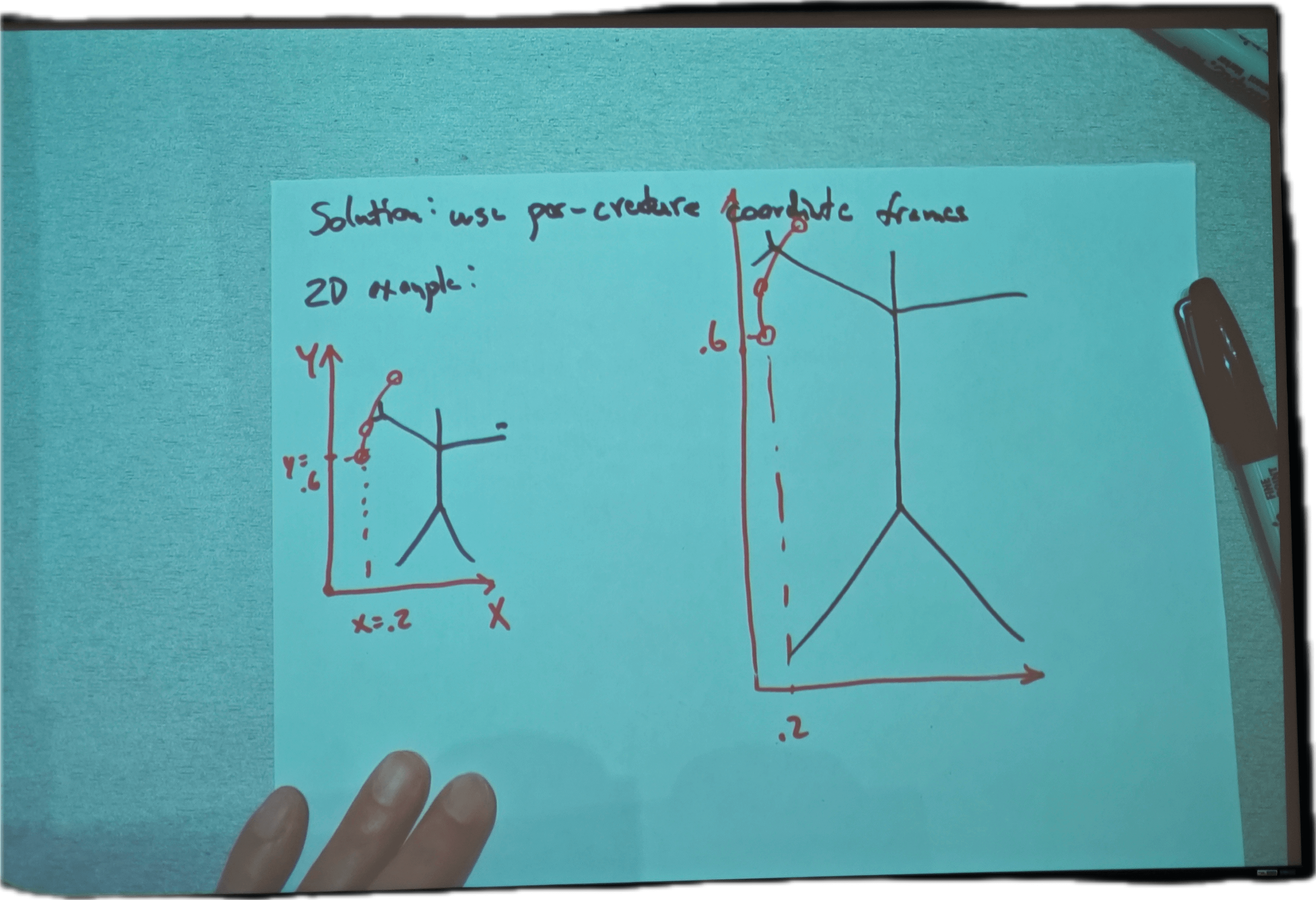
2. Moving Body Parts

Usually pose ends of limbs(IK) and rest of body follows.

Body parts locations are not in absolute coordinates.

Solution: use per-creature coordinate frames

2D example:

Coordinate frame from ground to grasper

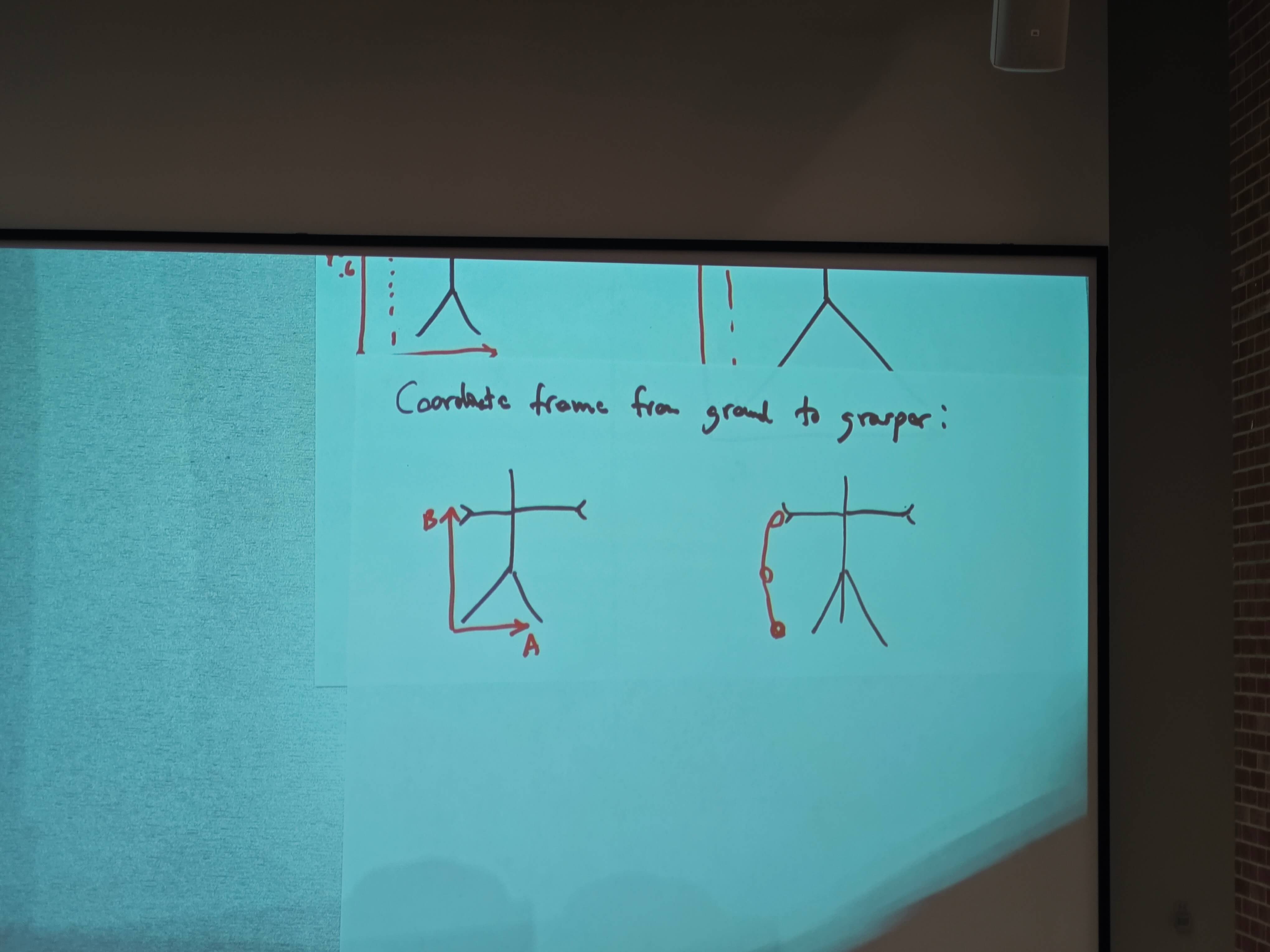
(pick up item from ground)

Align frame with object

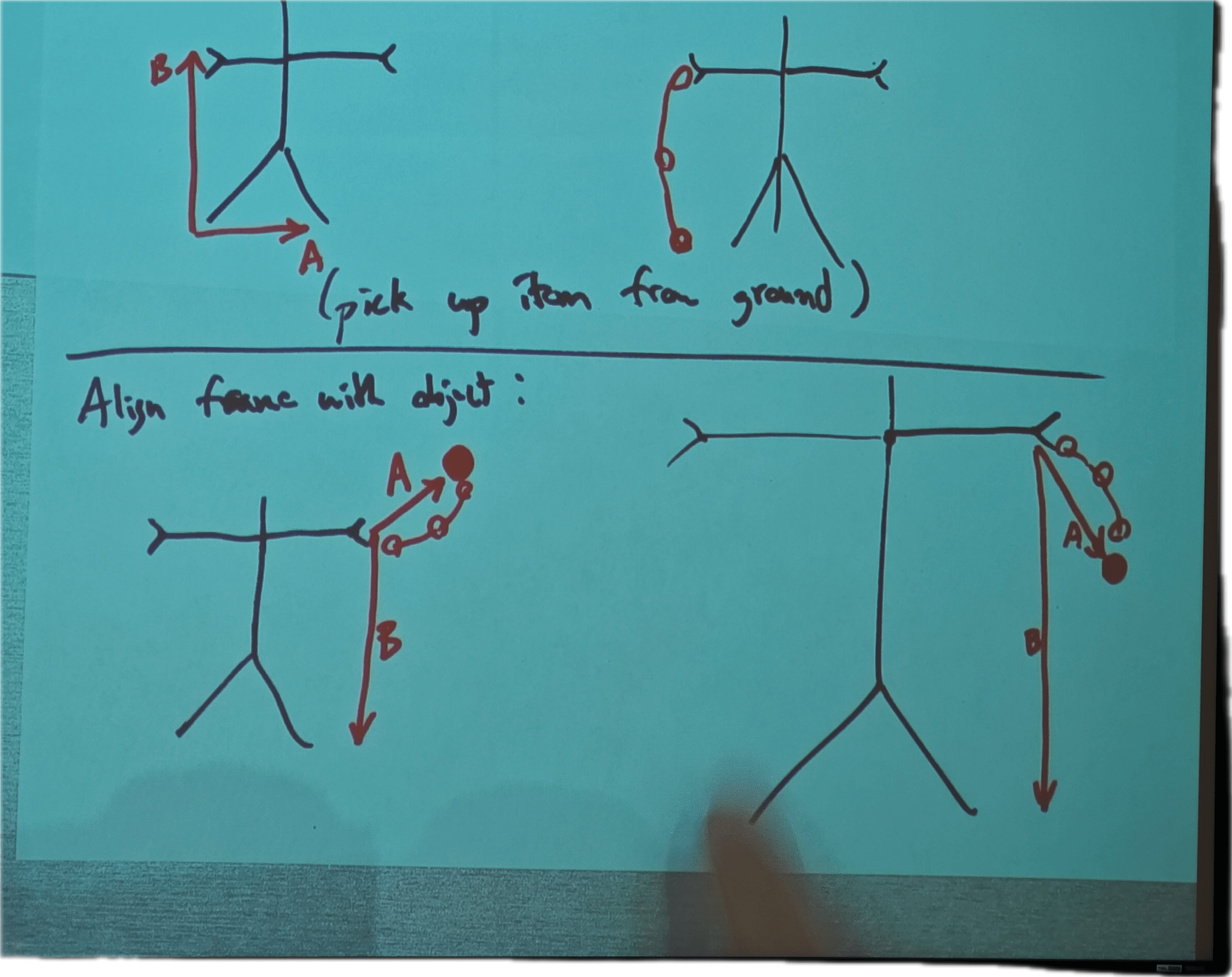
Align frame with mouth(for eating)

Particle System

Represent geometry as set of 3D points

+: (x,y,z), color, opacity, orientation, velocity, accelation

-: no connectivity, no surfaces,

Phenomena: smoke, water, fire, explosion, trees, grass, snow

Birth

randomly create particles

in a shape (box, sphere)
on a shape (sphere, mesh)

density of particles may be based on surface area or screen-space area

Intial Velocities: zero, outward from object, pseudo-random

1106

Particle State

Mass(m)

P=(Px,Py,Pz) position

V=(Vx,Vy,Vz) velosity

Many particles in a big list

Move them time in equal steps()

Simulation loop

For each timestamp
	For each particle i:
		Determine **forces** fi on particle
		Cacluate new velocity + position from fi
		Draw particle at postion pi

Posible froces

gravity
wind
damping
attraction to near particle
repulsion from other particle
spring attach to other particle (mass/spring simulation)

f: force

a: acceleration couple ordinary differential equation New velocity: v'

New position: p' Better

force of gravity(downward pointing vector) damping

Animal groups

Flocks, herds and schools: A distributed behavioral model

-Craig Reynolds, Siggraph 1987

flocks of birds
schools of fish
herds of wildebeests

Why fish?

defense against preditors

effective search for food

social & mating activity

efficient locomotion(drafting)

How to Animate?

keyframe each Ash? no!

simulate(roughly what animals do: observe & react)

Flight Model of Boid

has postion & velocity (6 degrees of freedom) DOF

min/max velocity

Flocking Behavior("forces")

Collision avoidance(with other boids, with obstacles)
velocity matching (near boids have similar velocityes)
flock centering - stay close to local center of flock mates
wander - small random divisition changes

1,2,3 - require knowing nearby boids

naive:

Behavior combining

Weighted averge of forces - sometimes leads to indecision

Better: prioritize some behaviors

behavior #1 makes a request

lefove acceleration used for behavior #2

Simulate Peception

vision
hearing
lateral line (fish: pressure)

Avoid Obstacle

Steer-to-avoid

intersect forward ray with world
Find silhouette point closet to the heading
aim one body length away from silhouette

Each boid is affected by closet boids (in neighborhood)

p's neighbors (k of them)

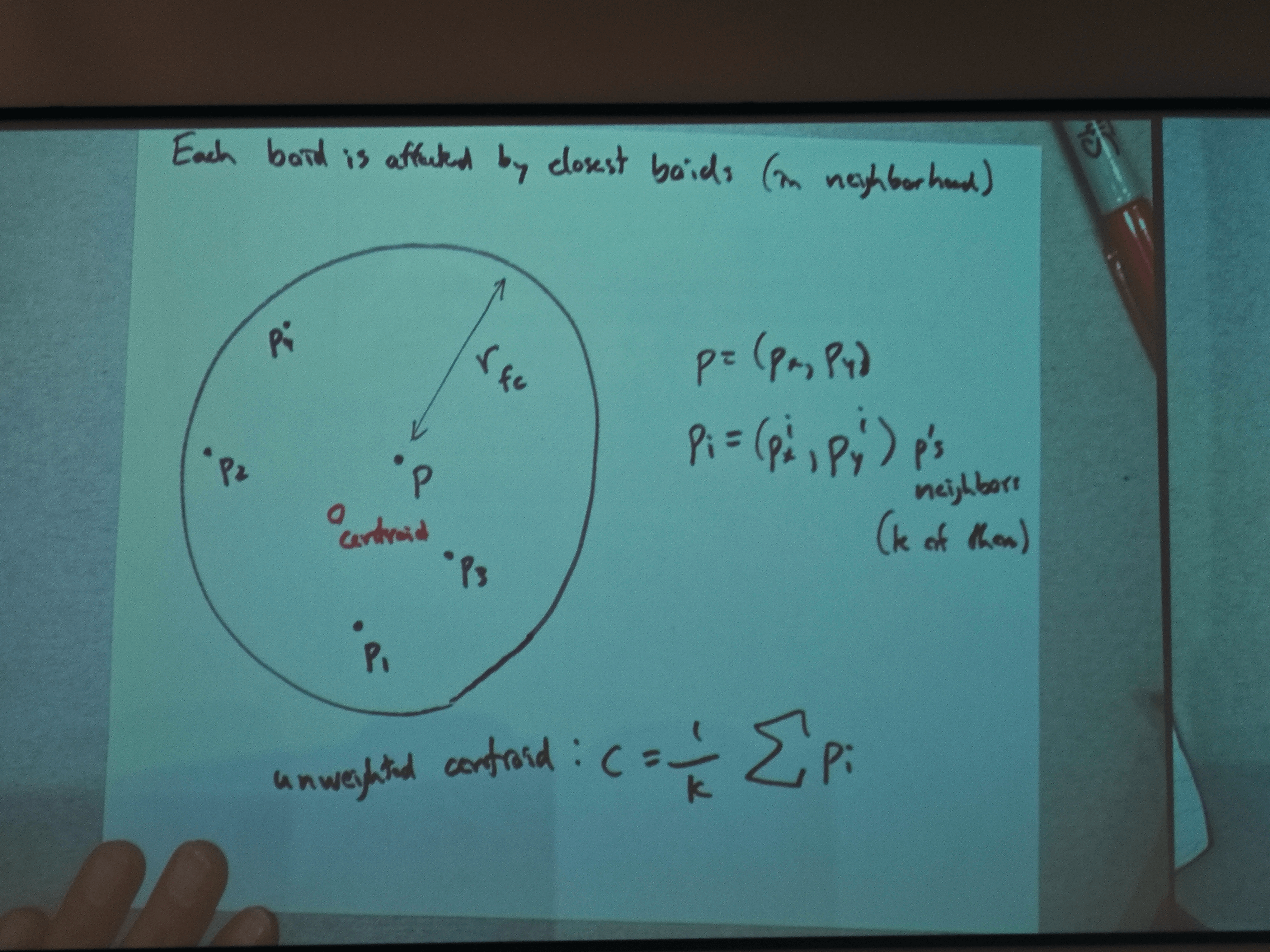
Unweighted centroid: c=

flock centering force

Problem：doesn't take int account p's position

distance between boids i&j Weights

(inverse square)

: tiny value

(linear)

weighted flock centering force (Normalize the weights)

Collision avoidence

repel when close

Velocity matching

Wander

Sum all forces

1111

Triffic Simulation

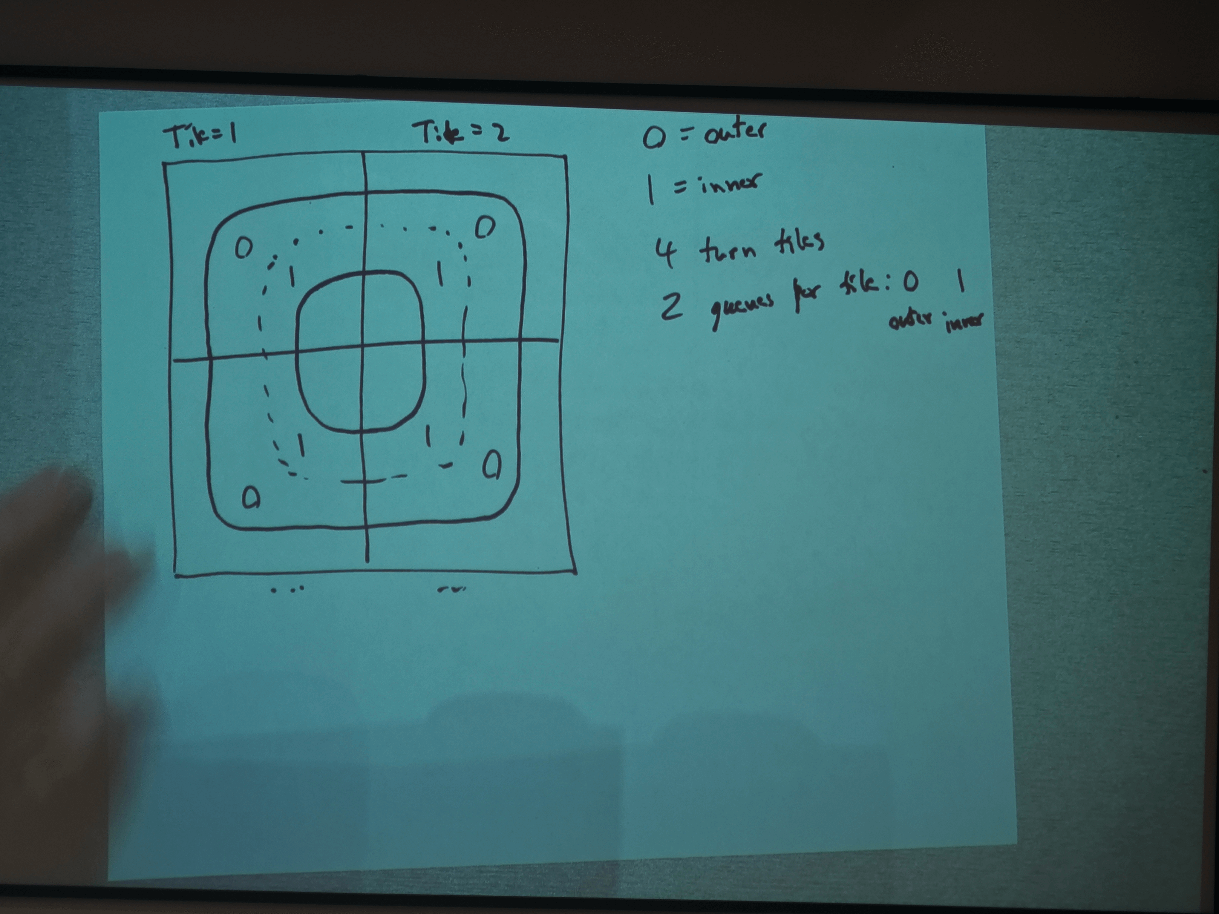
Turnning Tile

Outer Queue: empty

Inner Queue: A

When a car leaves queue of one tile, it enters queue of next tile

Each car can answer this: What other car is ahead of that one?
Possible answers
- car one some tile (check the queue)
- car on next tile (check que of next tile)
ignore cars further than one tile away

0 = outer

1 = inner

4 tunning tile

2 queues for tile:0(outer) 1(inner)

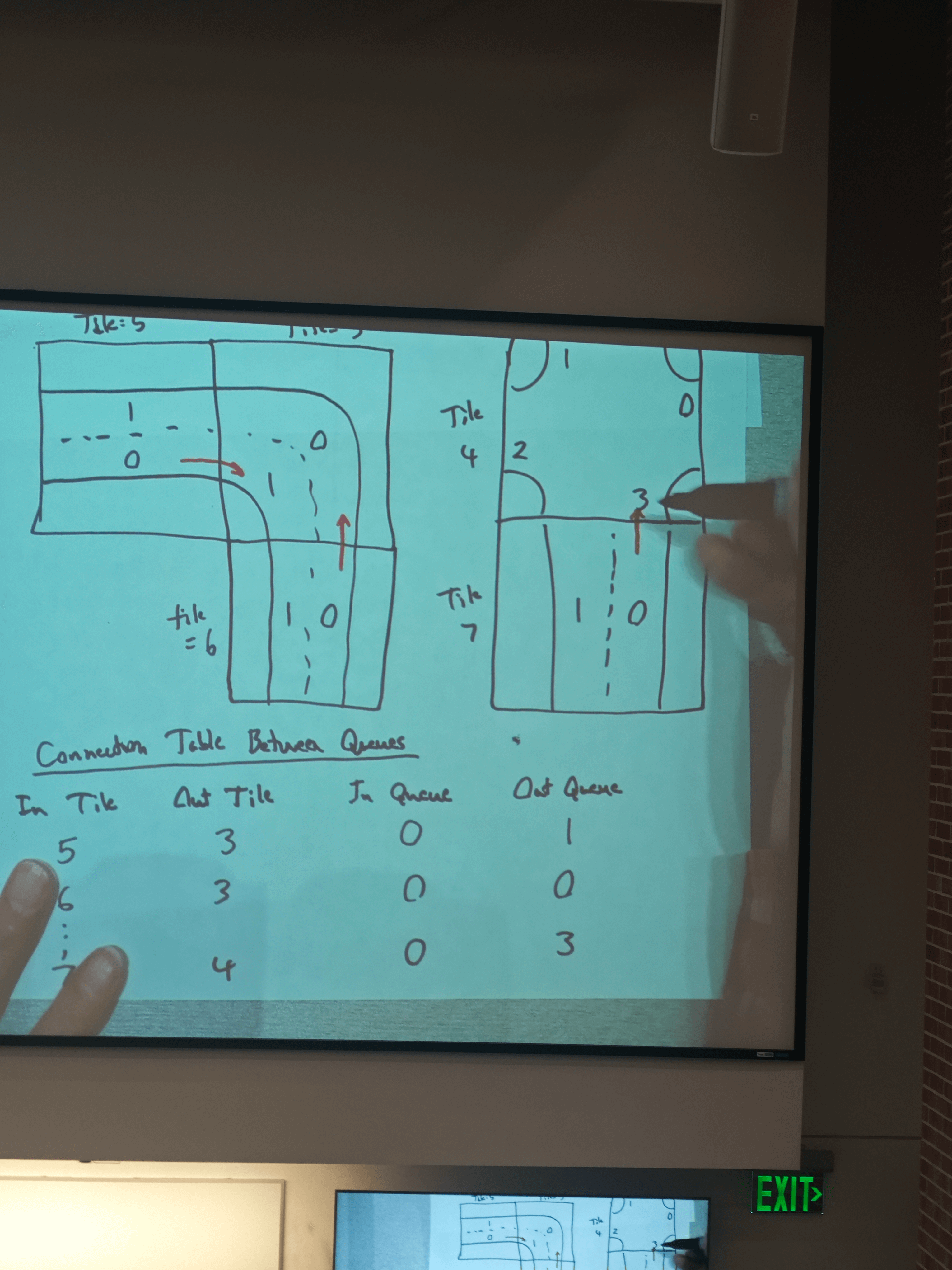
Connection Table Between Queues

In Tile	Out Tile	Out Queue
5	3	1
6	3	0
7	4	3

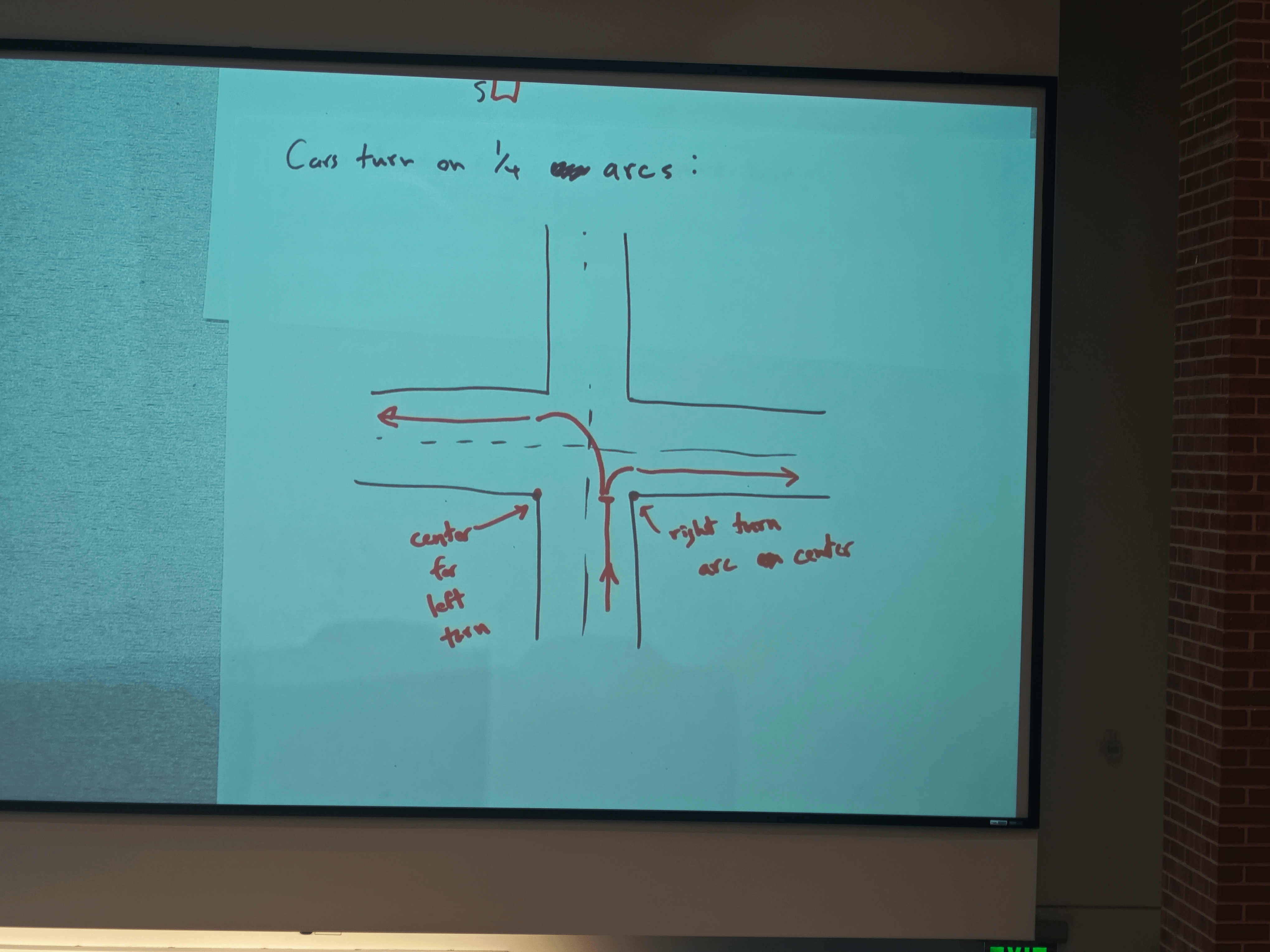
4 - Way Stop

Intersection has 4 car variables: was, west, north, south

N: empty

S: A

E: B

W: empty

Right- of way: first-come, first, serve basis

Can turn on 1/4 arcs

Slow down?

Create imaginary car ahead

Approach Traffic Test

one car on straight road
one car on loop
one car one road with intersection
Multiple cars on clasped loop
" " with intersection (3)

Car acceleration

Use Intelligent Driver Model(IDM)

Each car has several parameters

Symbol	Meaning	Common Values
	desired velocity	km
	mininum safe distance	m
	max acceleration	m/s
	comfortable deceleration	m/s
T	drivers response time	s
S	gap to next car

Each car calculates its current safe distance to next car

New acceleration

Crowds

In animation

pedestrians on street
armies on battlefield
people at outdorr concert

Similar do flocking but diferent

entirely 2D motion
characters have goal locations
may be tightly pecked
no local alignment with neighbors
lane formation

Two main Approaches

agent-based(fast, beahviors more local)
Potential field/continum-baseed (slower, behavior has more foresight)

A predictive Calltim Avoidence Model for Pestrian Simulation

Karamouzas, 2009

Agent-based

Per-Agent State

position
Orientation
velocity
radius

forces

attraction to goal position
repulsion from obstacles
avoidance of other agents

Attraction to Goal

is goal position
is speed preference
is time to reach speed pref
is direction to goal unit vector

Avoid Walls

is agents' radius
is normal at wall
agent's preferred to wall
shortest distance to wall
steepness of repulsion [1,4]?

Avoid other agents

confortable distanceo to others
dist between agents i& j
collision if

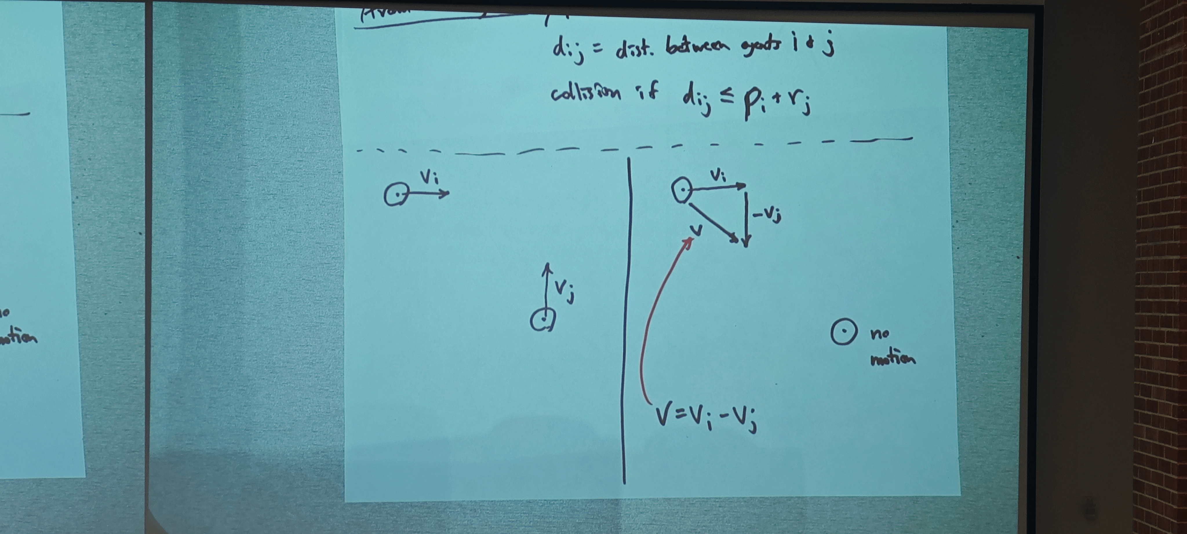
Position of agent i at time t (using v)

Collision will occur if/when

1113

some nearby avoidance forces ->

Continuum Crowds

Treuille et cl, Siggraph 2006

Charastics

Many characters share same goal (region)
Speed of agents based on average velocity of crowd
Speed varies with slope of terrain

Main Idea: Create "potential field" (artificial height) that guides agents with same goals

character "walking downhill"

1D example

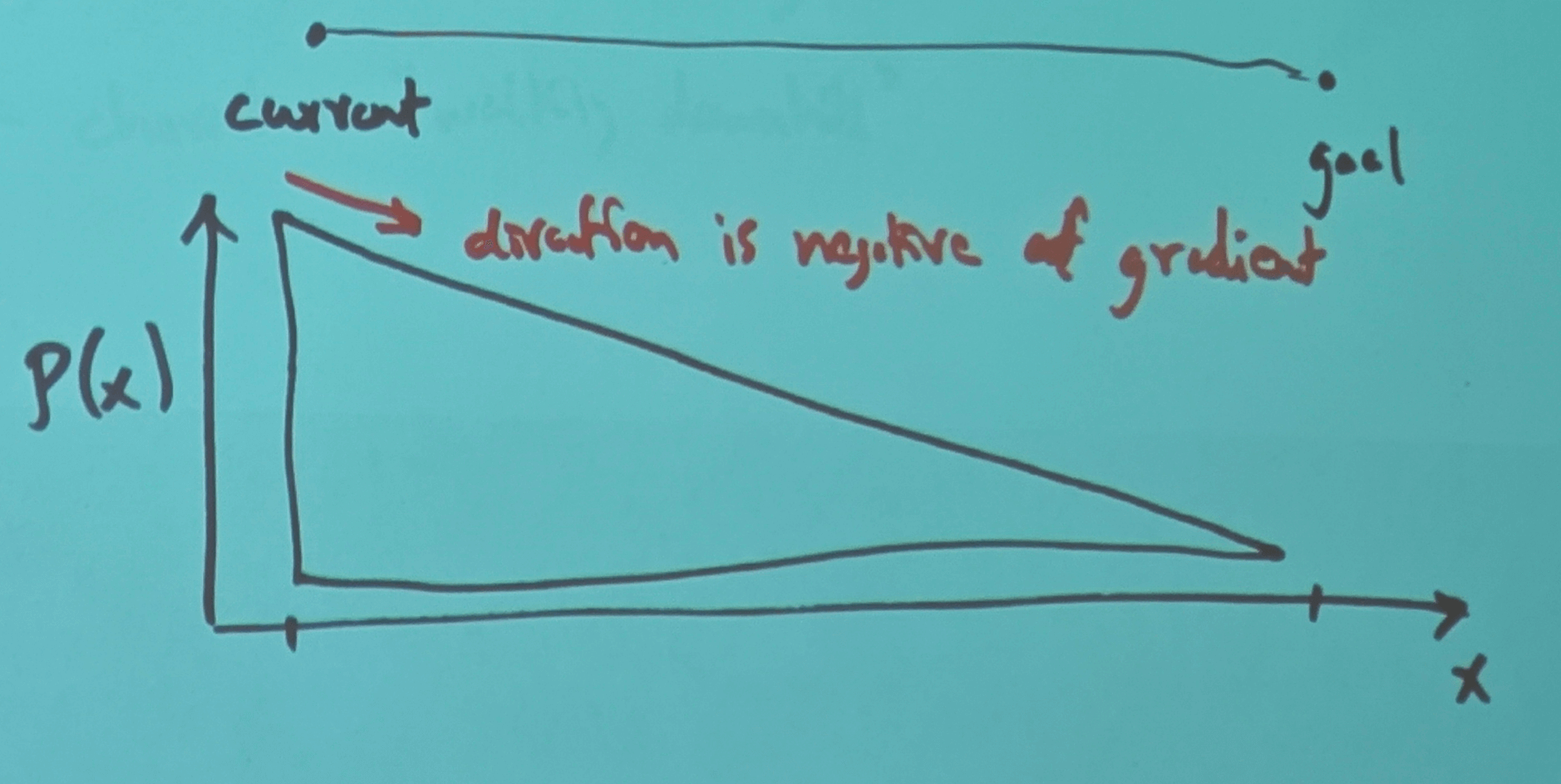
2D example

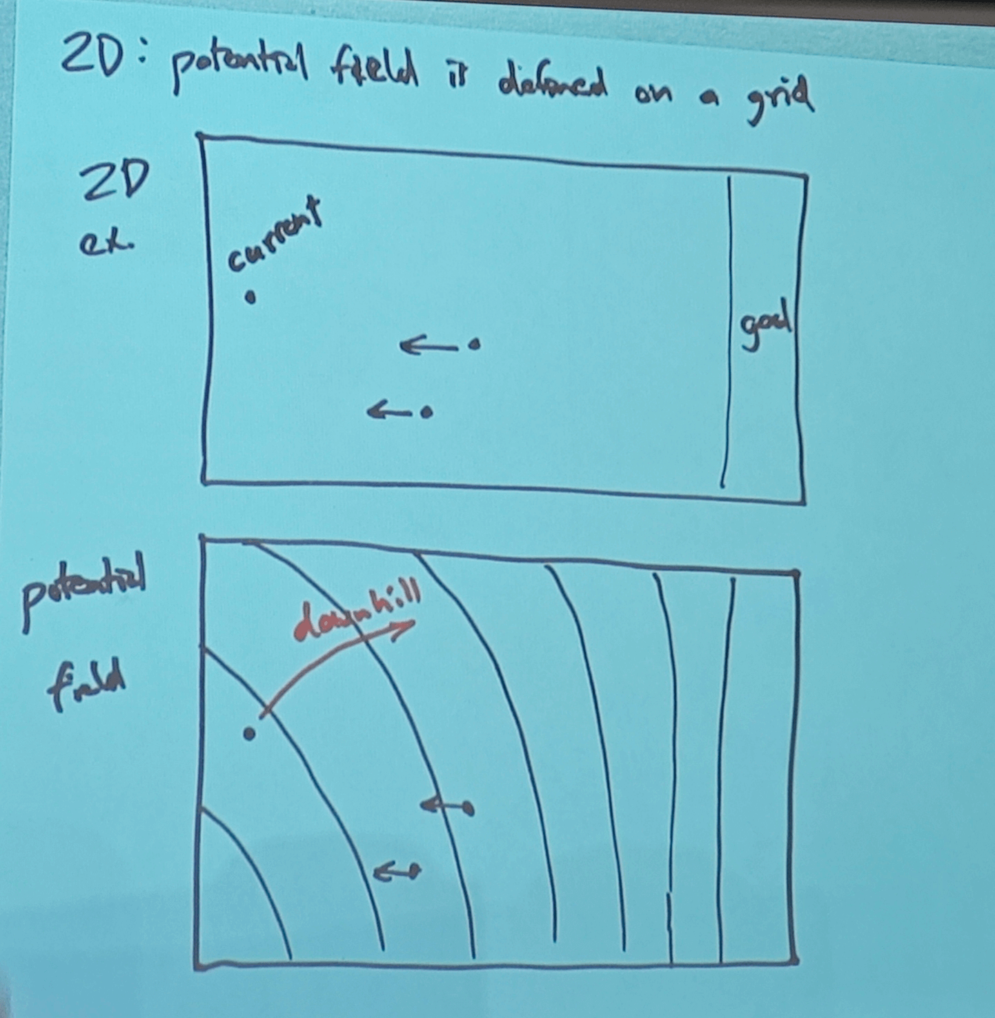
Potential is re-computed many times per second

Used by many agents

Result: lane following

Rouguelike Games

Berlin Elements

Random dungeon generation
Permadeath
Trun-based play(especially fights)
every action always available(non-modal)
Multiple ways to solve problems
Managing resources necessary to survive
Must fight to survive(hack and slash)
Items have different properties in different runs

1118

Minecraft: Voxel Worlds & Procedural Terrain

Voxel Representation

Minecraft represents the world using voxels (3D grid of blocks).

Each block:

fixed size
integer coordinates
block type (air, dirt, stone, water, grass…)
no deformation (not mesh surfaces)

Advantages

simple data structure
infinite world (extend grid as needed)
block-based gameplay (dig, place, build)
fast updates (modify a small part)

Chunks

To manage huge worlds, Minecraft groups voxels into chunks.

Typical size: 16×16×256 (x, z, y)
Allows:
- streaming
- parallel generation
- memory culling
- local updates

Only render chunks near the player.

Procedural Terrain: Noise Functions

Minecraft terrain height at (x, z) comes from Perlin/Simplex noise.

General formula:

1	height(x,z) = base + noise(x,z)*amp + biome_adjustment

Multiple Octaves

Use fractal noise: Creates:

mountains
plains
hills
caves (3D noise)

Biomes

Different regions use different noise parameters.

Examples:

desert → flat, sandy, no trees
forest → moderate height, trees
mountains → large amplitude noise
swamp → low, muddy, water patches

Biome = ruleset for:

block types
tree density
color
temperature / humidity
special features (cacti, snow)

Mesh Generation

Minecraft does not render each cube with 6 faces.

Too slow → millions of triangles.

Only render visible faces

If block A touches block B:

shared face is hidden → skip

So for each block, check 6 neighbors:

1 2	if neighbor is air: create quad for that face

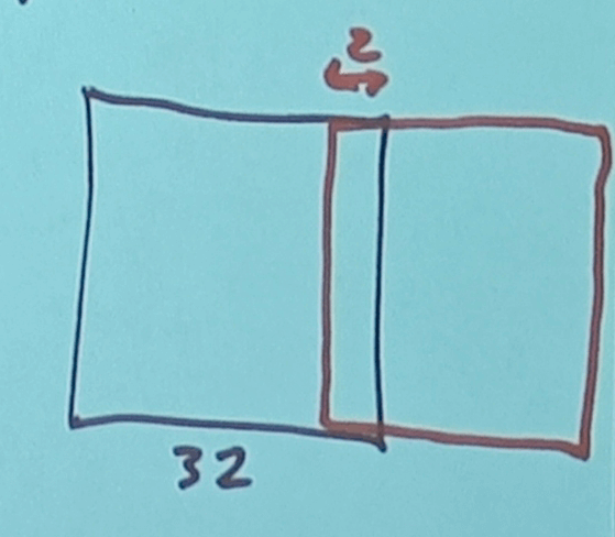
Greedy Meshing

Optimize mesh by merging adjacent faces with same material.

Instead of:

100 small quads

Use:

1 big quad

Benefits:

fewer polygons
fewer draw calls
faster rendering

Algorithm:

scan along axes
detect maximal rectangles of identical visible faces
emit large quad

Lighting (Block Light + Sky Light)

Minecraft uses light propagation, not per-pixel lighting.

Two components:

1. Sky Light

propagates downward from the sky
blocked by opaque blocks
used for day/night shading

2. Block Light

torches, glowstone, lava
propagated in BFS-like manner
decreases by 1 per block

Stored as integers (0–15).

Caves & Overhangs (3D Noise)

Using 3D noise:

if noise3d(x,y,z) > threshold:
    block = air (cave)
else:
    block = stone

Multiple layers:

Large caverns
Tunnels
Cliffs / overhangs (not possible with 2D heightmaps)

World Generation Pipeline

Choose biome
Compute terrain height using noise
Fill blocks up to height
Apply biome decorators:
- trees
- lakes
- ores
- villages
Generate caves
Build mesh with greedy meshing
Add lighting
Render chunk

Data Storage

Chunks saved as:

block IDs
metadata
compression (NBT format)

Allows incremental loading.

Summary

Minecraft's world is built from:

voxels stored in chunks
noise functions for terrain
biome rules for variety
greedy meshing to reduce polygons
light propagation for block lighting
3D noise for caves

Efficient, scalable, easy to modify → ideal for procedural generation.

1120

No Man Sky

Almost everything procedurally generated

terrain
creatures
planets
vehicles

Each planet described by 64-bit seed GDC videos

Sean Murray(2017) - noise, terrain
Innes Mckendrick(2017) - wrold creation (great!)
Grant Duncan(2015) - art for creatures & plants

Plant Terrain Concepts

3D voxel grid for terrain (not hight field)
voxels only in thin "shell"
sphere-to-cube projection
multiple noise technques
post-noise decorations

Terrain Shaped by Voxels - volume Elements(Cubes)

Each voxel: meter of volume
Voxles have material types: grass, rock, sand, etc
Stored in voxel chunks, represent overlap no cracks

Each voxel

density (2 bytes)
material type (2)
material blend (2)

Use dual contouring to make polys(polygons)

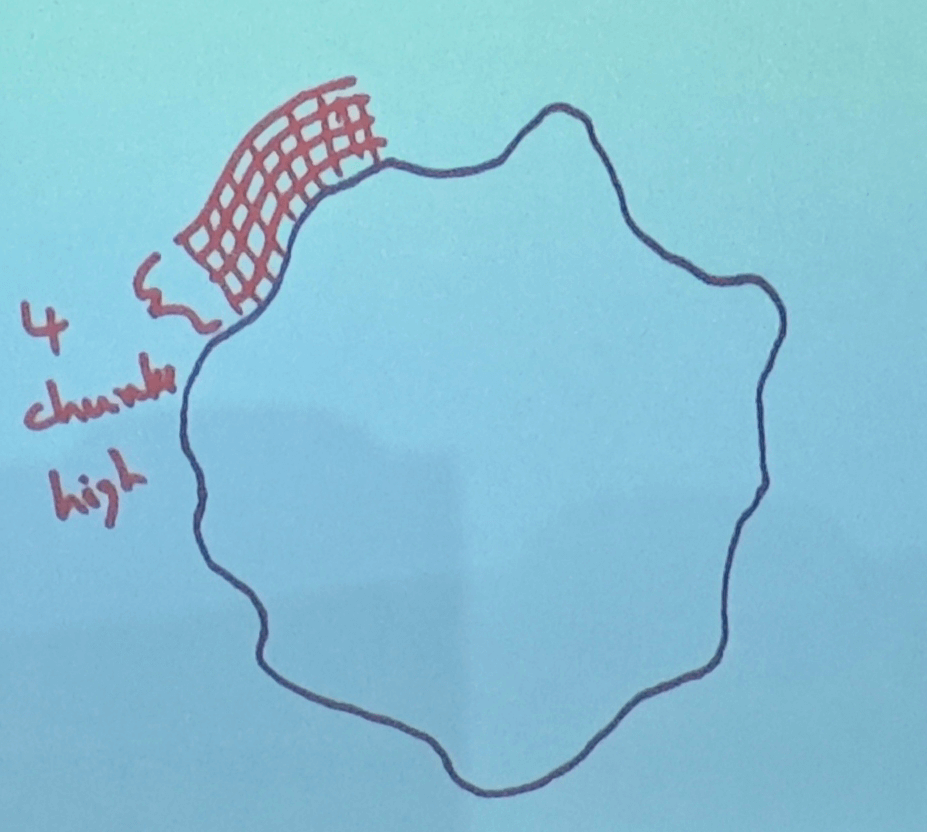
Terrain Shell

Voxels in layer that is 128 meters thick (4 chunks)
Rides on top of low-frequency noise layer (height field)
Height can vary by 1km
High mountains, deep oceans

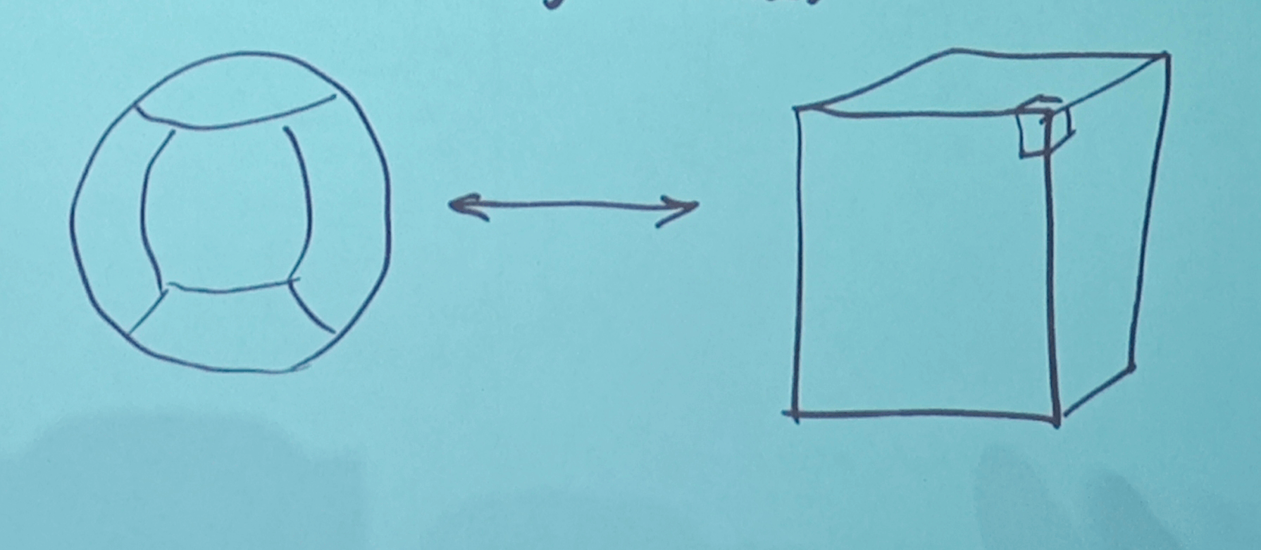
Sphere to Cube

Voxels placed on a curved sphere in game

For storage, indexed on grid(cube)

Deorations

rocks
rock worms
caves
pilers(enery source)
plants

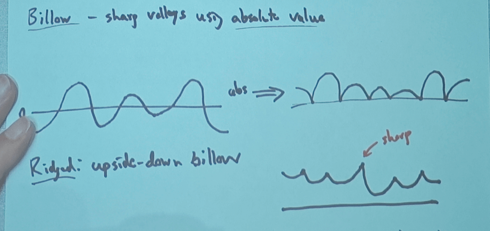
Multiple Noise Methods

sum of perlin octaves(fractal noise, fractal Brownian motion, octave noise)

Billow - sharp valleys using absolute value

Ridged: upside-down billow

Domain warping (like Minecraft): add noise to input position

Attribute Cascade

Galaxy - Emty/Harsh/lush/Normal

Star System Spectal Class: Yellow/ Red/ Green (not real)/ Blue

Planets

Terrain/Biomes largely independent Terrains: Ocean Worlds -Continent, Pangea - Swamp -Riverland

Plants& Animals

Animals

Locomotion vareidy: walk,fly, swim, ...

usual graphics component:

mesh
rig(skleton)
textures

artist creates base model

Skeleton (rig)
mesh geometry (z- brush or simulator)
bone scaling system -> changes the rig

animation rig shared across animals:

cows
horses
antelope

swim: same rig

dolphin
shark
whale

decorations: Fins, tail, dorsel crest, spikes, etc

large techure library - cretve skins

Plants

trunks shared between trees

different branches added

Leaves & materials

bone scaling for different shapes(bend...)

library at bark & textures

1125&1202

Generative AI

What is Generative AI?

A model that produces new data resembling the data it was trained on.

Generates:

text
images
3D shapes
audio / music
code
terrain / textures (PCG!)

Instead of predicting labels (discriminative), it generates samples (generative).

Discriminative vs Generative

Discriminative

Learns the boundary:

Examples:

classifier
segmentation model
logistic regression
ResNet for ImageNet

Generative

Learns the distribution of data:

Examples:

GPT (next-token prediction)
Diffusion models
GANs
VAEs

Large Language Models (LLMs)

LLMs are trained using next-token prediction:

Transformer architecture

Key components:

self-attention
multi-head attention
positional encoding
feed-forward layers

Properties:

learns long-range dependencies
massive scalability
parallelizable (unlike RNNs)

Diffusion Models

Modern SOTA for image generation.

Forward process

Add noise gradually:

1	x₀ → x₁ → … → x_T (pure noise)

Reverse process

Learn to denoise:

1	x_T → x_{T-1} → … → x_0

The model predicts either:

the denoised image
the noise itself
velocity / score function

Why Diffusion Works Well

stable training
excellent mode coverage (no mode collapse like GANs)
conditioning is easy (text, masks, depth)
supports image editing (inpainting, outpainting)

Latent diffusion (Stable Diffusion):

compress image into latent space
run diffusion in latent → faster, cheaper

GANs (Generative Adversarial Networks)

Two networks:

Generator G: produces fake samples
Discriminator D: distinguishes real vs fake

Train in a minimax game: Pros:

sharp images
fast inference

Cons:

unstable training
mode collapse

VAEs (Variational Autoencoders)

Encode → latent → decode.

Latent is sampled from Gaussian distribution.

Objective: Pros:

structured latent space (good for interpolation)
stable training Cons:
blurry images

Generative AI in Games (PCG)

Used for:

terrain generation
textures (style transfer, diffusion)
creature/weapon/item variation
dialogue / quest generation (LLMs)
animation synthesis
NPC behavior
procedural sound generation

Why generative models help PCG

infinite variety
controlled randomness
artist-guided generation
faster content pipeline

Prompting & Conditioning

Models can be guided by:

text prompts
images
sketches
depth maps
segmentation masks
engine metadata (for game content)

Control techniques:

classifier-free guidance
ControlNet
LoRA (lightweight fine-tuning)
inpainting masks

Risks & Limitations

hallucination
copyright concerns
bias in training data
safety alignment
compute cost
unpredictable outputs

But rapidly improving with:

RLHF / RLAIF
synthetic data refinement
guardrail models

Summary

Generative AI includes:

LLMs for language
Diffusion models for images
GANs / VAEs for latent modeling
Transformers everywhere

And is heavily used in:

PCG
game asset creation
animation
world generation

本文链接： https://20021123.xyz/2025/12/10/cs8803-Procedural-Content-Generation/

版权声明： 本博客所有文章除特别声明外，均采用 CC BY 4.0 CN协议许可协议。转载请注明出处！

不知不觉Never Settle

Never Settle